Microsoft Excel’s “Autofit” feature is essential for optimizing the visibility of data within a spreadsheet. By default, Excel cells are set to a standard size, which often proves insufficient for longer text entries or larger numbers. Autofit comes into play by dynamically adjusting the height of rows and the width of columns to accommodate the size of the content within, ensuring that all data is visible and neatly presented without manual resizing.
To access the Autofit feature, users can employ several methods, including the use of mouse actions, the Excel ribbon, and keyboard shortcuts. The mouse double-click method is a quick and intuitive way to autofit rows and columns by simply double-clicking on the boundary of a cell. For more structured adjustments, the Excel ribbon offers an “Autofit Column Width” or “Autofit Row Height” option under the “Format” menu in the “Cells” group on the “Home” tab. Keyboard enthusiasts can make use of shortcuts such as “ALT + H + O + I” for columns and “ALT + H + O + A” for rows, providing a fast, no-mouse-required alternative.
How to AutoFit Column Width in Excel via Cell Labels
This method is tailored for those who prefer a hands-on approach to adjusting column widths in Excel. By directly interacting with the column labels at the top of your spreadsheet, you can quickly and efficiently resize columns. This approach is especially useful for making on-the-fly adjustments to individual or multiple columns, ensuring that all content is properly displayed without cutting off any text or numbers.
-
Manually Adjust Width
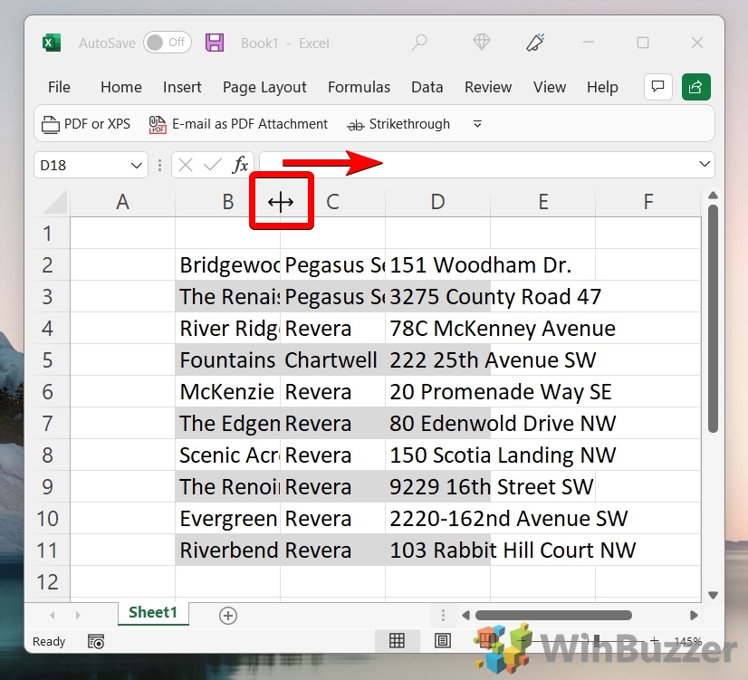
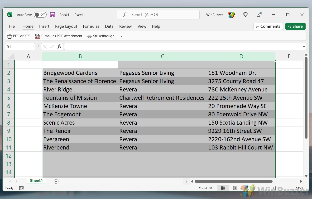
To manually adjust the width of a column, hover your cursor over the column divider until it turns into a double-sided arrow. Click and hold, then drag the divider left or right to decrease or increase the width of the column, respectively. This method allows you to customize the column width based on your visual preference or specific content needs.

-
AutoFit Column Width
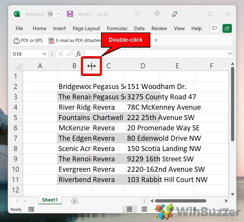
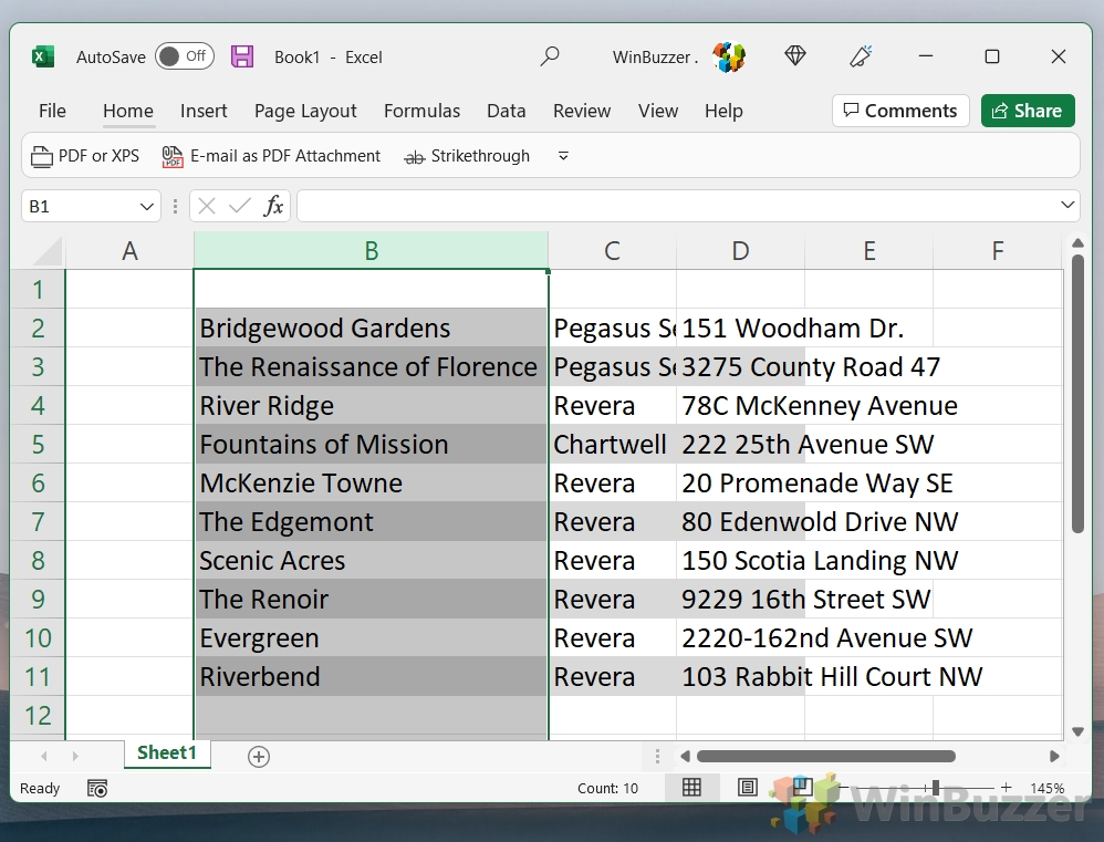
For an automatic adjustment, position your cursor on the right-hand divider of the column header until the cursor changes to a double-sided arrow. Double-click, and Excel will automatically resize the column to accommodate the widest piece of content. This feature is particularly useful when you have long headers or data entries that exceed the default column width.

- Your cell will automatically resize to fit your number or text

-
AutoFit Multiple Columns
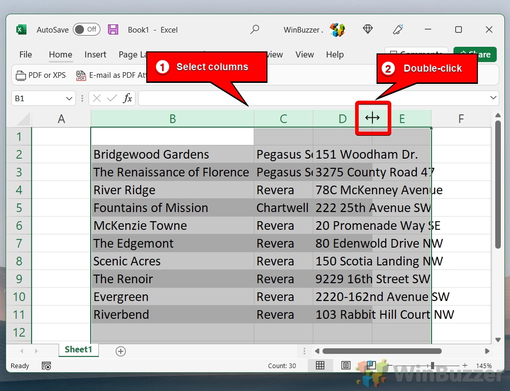
To auto-size several columns at once, click and drag across the column headers of the columns you wish to adjust, or hold the Ctrl key and click on individual non-adjacent column headers to select them. After selecting, move your cursor to the right-hand border of any selected column header and double-click.

- Excel will adjust your selected columns to fit
All selected columns will resize to fit their longest pieces of content, ensuring consistency across your data presentation.

-
AutoFit All Columns
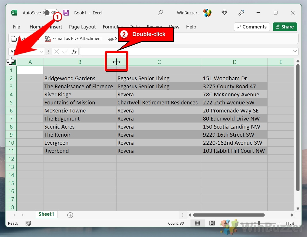
To apply autofit to every column in your worksheet, click the select-all button located at the top-left corner of your worksheet (where the column headers and row numbers meet). This selects the entire worksheet. Then, double-click the divider of any column header. Excel will auto-adjust every column in the sheet to fit its content, optimizing the visibility of your entire dataset with a single action.

How to AutoFit Row Height in Excel
Adjusting the row height is crucial when dealing with content that varies in size, such as multiline text entries or cells with larger font sizes. This method focuses on ensuring that the row height accommodates all content within a cell, making everything visible at a glance without the need for manual scrolling or resizing.
-
Adjust Row Height
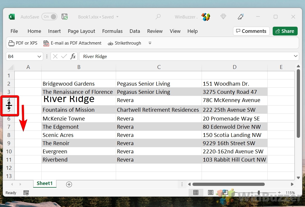
To change a row’s height, move your cursor to the bottom border of the row number until it becomes a double-sided arrow. Click and drag up or down to decrease or increase the row’s height. For an automatic adjustment, double-click the bottom border of the row number. Excel will automatically resize the row height to accommodate the tallest content in the row, ensuring that all data within the row is fully visible without scrolling.

How to AutoFit Columns and Rows in Excel via the Ribbon
For users who prefer navigating through Excel’s menu system rather than interacting directly with the sheet, autofitting columns and rows via the ribbon is an ideal method. This approach allows for precise control over the autofit process, utilizing Excel’s built-in formatting options.
-
AutoFit Row Height
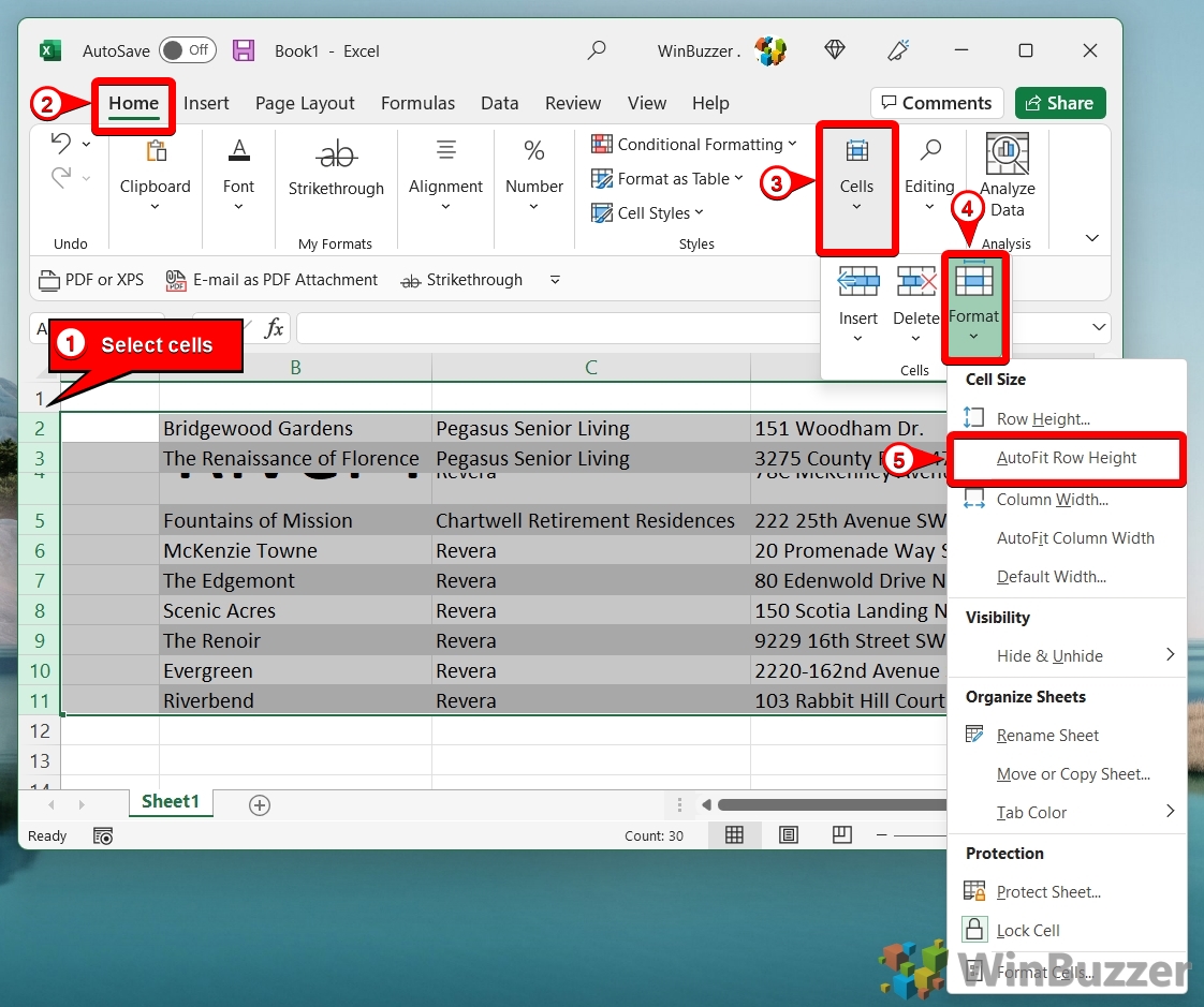
Begin by selecting the rows you wish to adjust. You can do this by clicking on the row numbers to the left of your sheet. Then, navigate to the “Home” tab on the ribbon, click “Format” within the “Cells” group, and choose “AutoFit Row Height“.

- Excel will adjust your row heights to fit the tallest content
Excel will analyze the content of the selected rows and automatically adjust their height to ensure that the tallest content in each row is fully visible, thus eliminating the need for manual row height adjustments.

-
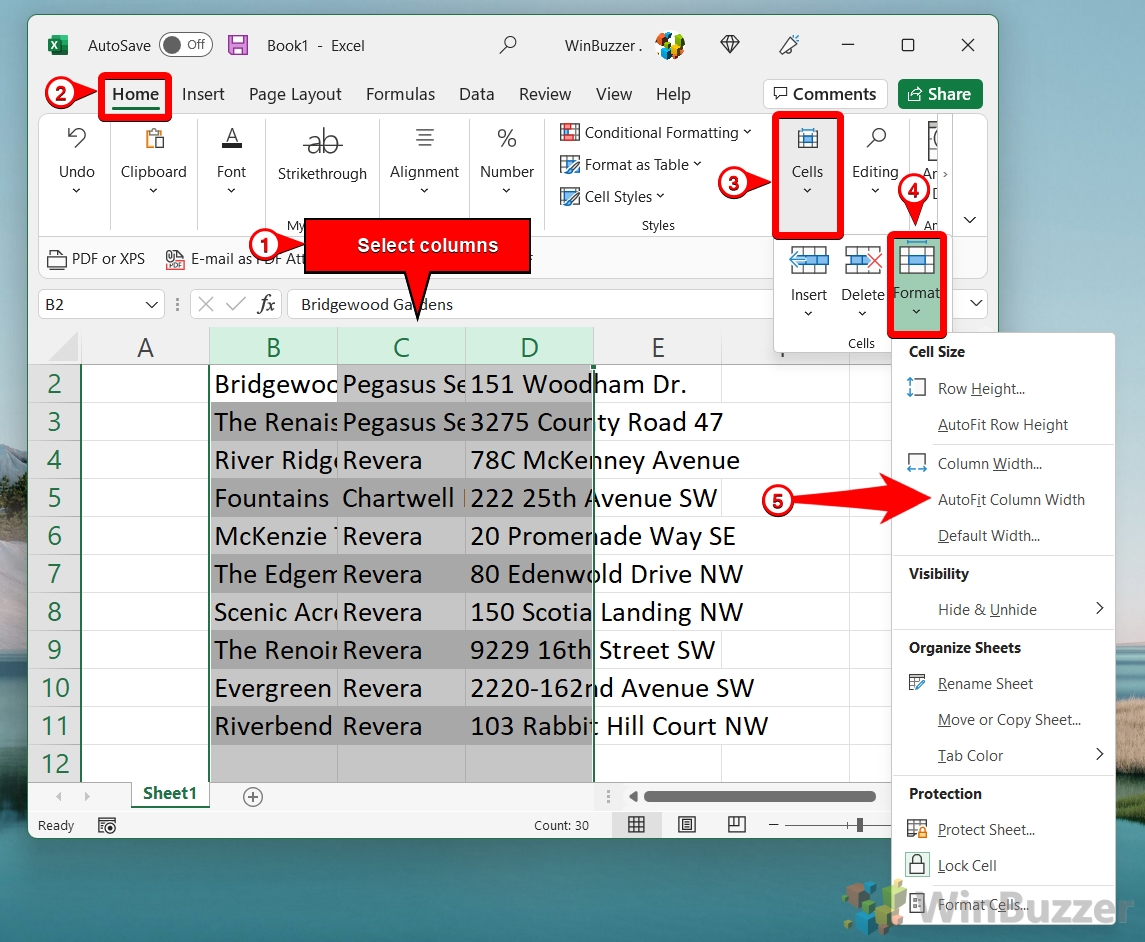
AutoFit Column Width
Select the columns you intend to adjust by clicking on their respective column headers. Once selected, go to the “Home” tab, find the “Cells” group, and click “Format“. From the dropdown menu, select “Autofit Column Width“.

- Excel will autofit your columns to the content in them
Excel will resize the selected columns so that each one is wide enough to display the longest piece of content within that column, ensuring data is clearly visible across your worksheet.

How to Use the Excel Autofit Shortcut
For the power user looking to streamline their workflow, Excel offers keyboard shortcuts for autofitting rows and columns. This method is all about efficiency, allowing you to quickly resize cells to fit their content without taking your hands off the keyboard. It’s ideal for users who work extensively with Excel and are familiar with shortcut keys.
-
Use Shortcuts for AutoFit
To quickly autofit columns, first select the columns you wish to adjust by clicking on their headers. Then, press “Alt + H” to select the Home tab on the ribbon, followed by “O” to open the Format menu, and finally “I” for autofitting the column width.
For rows, after selecting them by clicking on the row numbers, use the same combination but replace “I” with “A” to autofit row height. These shortcuts allow for rapid resizing of rows and columns, streamlining your workflow in Excel.

FAQ – Frequently Asked Questions About Excel Autofit
What is the shortcut key to arrange rows and columns in Excel?
To quickly autofit the row height, select the rows you want to adjust, then press “Alt + H” to select the Home tab on the ribbon, followed by “O” to open the Format menu, and “A” for autofitting the row height. For autofitting column width, select the columns and press “Alt + H”, then “O”, followed by “I”. This sequence of shortcuts activates Excel’s autofit feature without the need for mouse navigation.
How do I sort Excel columns alphabetically and keep rows together?
Sorting columns alphabetically while keeping the rows intact can be achieved through Excel’s Sort functionality. After selecting the range of data or the entire column you want to sort, navigate to the “Data” tab on the ribbon and select “Sort”. In the dialog box that appears, ensure that the “My data has headers” checkbox is selected if your data includes headers, and choose the column you want to sort by. Excel will then reorder the columns alphabetically without disrupting the row structure.
How do I resize a table in Excel without losing formatting?
To resize a table in Excel without losing formatting, adjust the column widths and row heights by dragging the borders between headers or by using the autofit function, which preserves cell formatting. To do this without dragging, you can select the table, right-click on a row or column header, choose “Column Width” or “Row Height”, and input your desired dimensions. This method ensures that the table resizes without altering cell formats like font size, cell color, or borders.
How do I AutoFit rows in Excel?
To autofit rows in Excel and ensure that all content is visible, select the rows you wish to adjust, either by clicking and dragging across the row numbers or by using the “Ctrl” key for non-adjacent rows. Once selected, navigate to the “Home” tab, click “Format” within the “Cells” group, and select “AutoFit Row Height”. Excel will then automatically adjust the row height to accommodate the tallest content in each row, which is particularly useful for rows containing wrapped text or varying font sizes.
How do you make Excel cells expand to fit text automatically vertically?
For cells to automatically expand and fit text vertically, first ensure that the text wrapping feature is activated by selecting the cells, right-clicking, choosing “Format Cells”, and checking “Wrap Text” under the Alignment tab. Then, use the autofit feature by positioning the mouse over the bottom border of the row number until the cursor changes to a double-sided arrow and double-clicking. This action prompts Excel to expand the row height to display all wrapped text fully.
How do I sort multiple columns in sheets without mixing data?
In Google Sheets, to sort multiple columns while maintaining data integrity, highlight the range of cells that includes all columns you intend to sort. Then, navigate to “Data” in the top menu and select “Sort range”, ensuring that you check “Data has header row” if your range includes headers. Specify the column to sort by and the sort order. This will rearrange the columns in the desired order without disassociating the rows from one another.
How do you AutoFit all columns rows instantly?
For an instant autofit of all columns and rows in an Excel worksheet, click the select-all button at the intersection of the column and row headers to highlight the entire sheet. Then, position your cursor at the edge of any column header until it turns into a double-sided arrow and double-click to autofit all columns. Repeat this action at the bottom of any row header to autofit all rows, making the cells adjust to the content size immediately.
What is the code for AutoFit in Excel VBA?
In Excel VBA, the autofit method can be applied to a range of cells, entire columns, or rows. For instance, to autofit column A, use Columns(“A:A”).AutoFit. For multiple columns, you can specify a range like Columns(“A:C”).AutoFit. Similarly, to autofit row heights for rows 1 through 3, the code would be Rows(“1:3”).AutoFit. These lines of code can be incorporated into macros to automate the resizing process for efficient data display.
Why are my rows not auto-sizing in Excel?
If your rows in Excel are not auto-sizing, it could be due to several reasons: merged cells, which can interfere with the autofit functionality; presence of manual line breaks (inserted with Alt+Enter) within the cells; or the wrap text feature might not be enabled. To troubleshoot, ensure there are no merged cells within the rows you’re trying to autofit, enable wrap text if needed, and remove any manual line breaks. If these steps don’t solve the problem, checking cell formatting or using VBA scripts to adjust row height might be necessary.
How do you distribute rows and columns evenly in Excel?
To evenly distribute rows and columns in Excel, first select the rows or columns you wish to equalize. Right-click on the selected header(s) and pick “Row Height” or “Column Width” from the context menu. Enter a specific measurement to set them to a uniform size, which will distribute them evenly across the selected range. This method is particularly useful for standardizing the layout of your spreadsheet, separate from the content-based autofit feature.
How do I resize all rows to a specific height?
To set all rows to a specific height, you’ll need to select the entire sheet by clicking the top-left corner between the row numbers and column letters, or by pressing “Ctrl + A”. Right-click on one of the selected row numbers and choose “Row Height” from the dropdown menu. In the Row Height dialog box that appears, type in your desired height, and all rows will update to reflect this new dimension.
How do I resize a column or row in Excel to best fit the contents?
To resize a column to best fit its contents in Excel, hover your cursor over the right-side edge of a column header until it changes to a double-sided arrow and double-click. Excel will then adjust the column width to accommodate the longest piece of data in the column. For rows, double-click the bottom edge of the row header after the cursor changes to a double-sided arrow to automatically resize the row height to fit the tallest content within the row.
How do I make all columns the same width in sheets?
In Google Sheets, to standardize the width of all columns, click on the gray square at the top-left corner to select the entire sheet, or click and drag across the column headers to select specific columns. Right-click on any selected column header and select “Resize columns”, followed by entering the desired pixel width. This will uniformly set the width of all selected columns, ensuring consistency in your spreadsheet’s appearance.
What is the formula to AutoFit row height in Excel?
While there’s no direct formula within Excel for autofitting row height, you can use the following VBA code to achieve this: ActiveSheet.Rows.AutoFit. Incorporate this line into a macro to autofit the row heights across the entire active sheet. This is useful for applying autofit to multiple rows simultaneously, especially when dealing with large datasets or dynamic data ranges.
Can Excel handle large data sets and what’s the best way to AutoFit columns and rows for them?
Excel is capable of handling large datasets, though performance might slow down with very large volumes. When dealing with extensive data, it’s more efficient to use the “Format as Table” feature, which provides better performance and automatically applies autofit to table columns as you input or update data. Additionally, for large datasets, you might consider using VBA scripts to autofit in batches, reducing the processing load on Excel.
Related: How to Move or Swap Columns in Excel
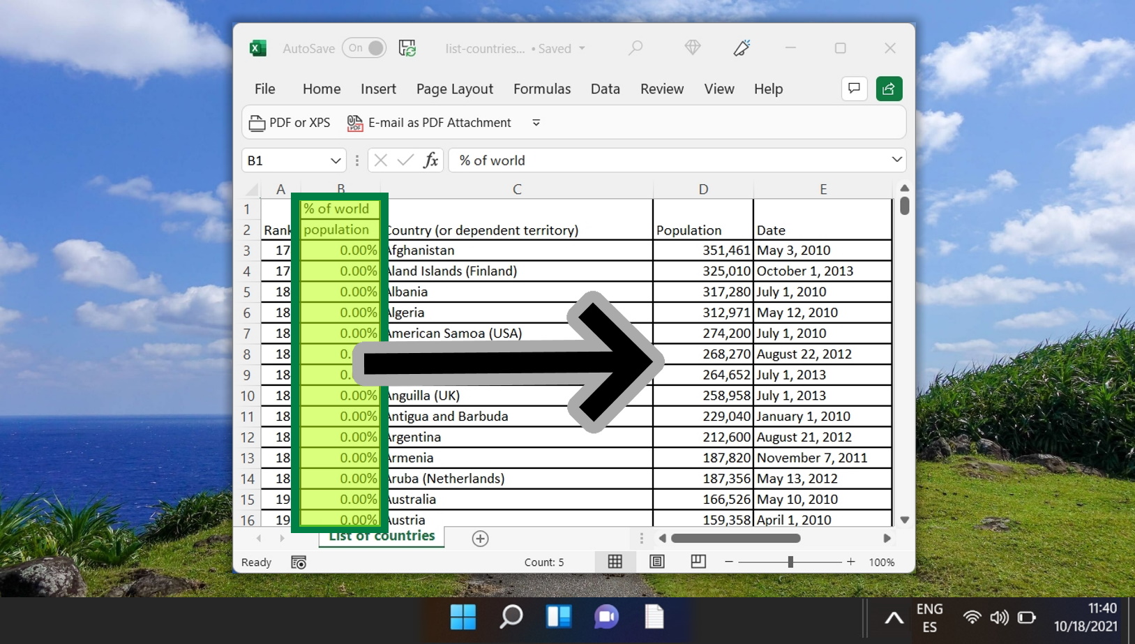
In a perfect world, you’d never need to rearrange columns in Excel. Planning a spreadsheet in advance should save you from having to perform large-scale rearrangement of your documents. The world isn’t perfect though, and the chances are that you’ll think of better ways to layout your spreadsheet or receive additional information to integrate.In our other guide, we show you how to move or swap columns in Excel.
Related: How to Remove Spaces in Excel
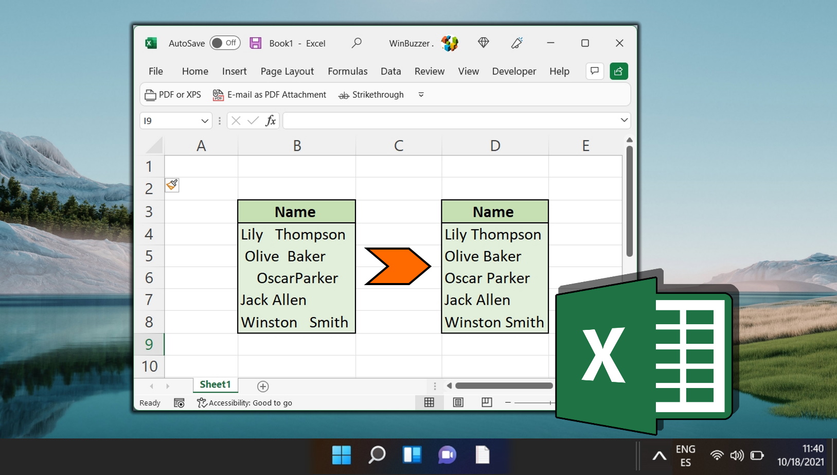
When managing extensive datasets in Excel, ensuring data consistency is crucial. An all too common inconsistency is unwanted spaces — whether they creep in at the beginning or end of a text string, appear as unwarranted gaps between words, or are unintentional space characters throughout your content. In our other guide, we show how to use the Replace Feature, the TRIM funcion, and the SUBSTITUTE function to seamlessly eliminate unwanted spaces in Excel.
Related: How to Add Shading to Alternating Rows in Excel
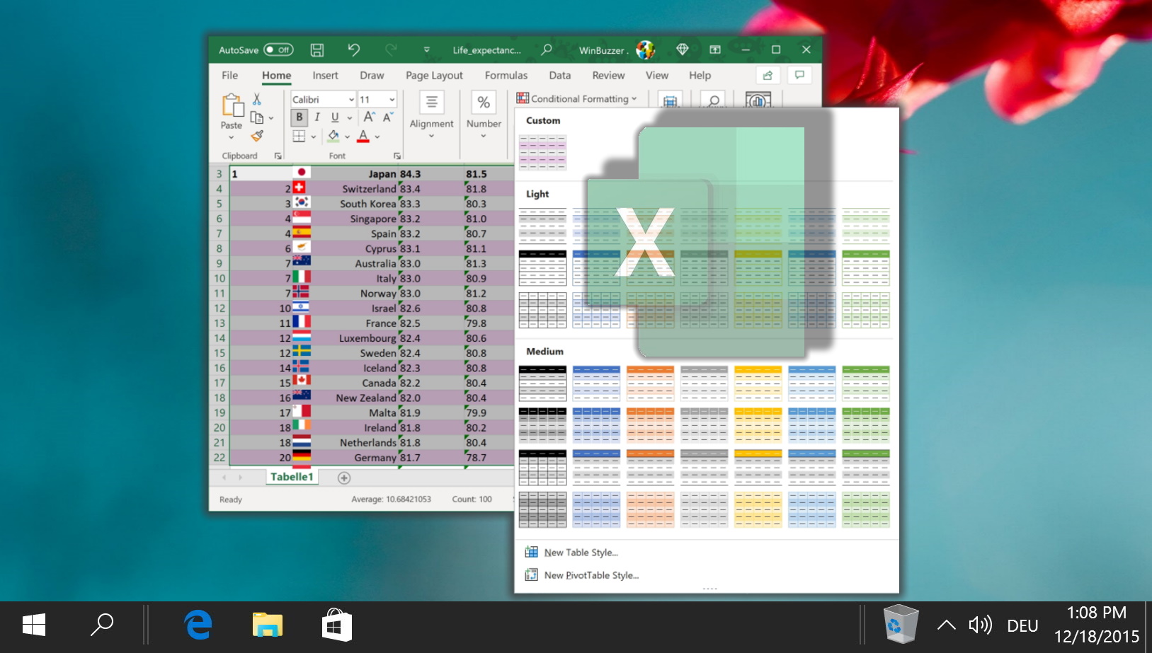
It’s an old trick at this point, but applying shading (zebra stripes) to alternative rows in Excel makes your sheet easier to read. The effect, also known as banded row, allows your eyes to keep their place more easily when you’re scanning a spreadsheet. The difficulty, then comes in knowing where to look and how to format cells as a table in the first place. In our other guide, we show you how to apply and customize table formatting to form alternating rows in Excel.
Last Updated on April 22, 2024 10:43 am CEST by Markus Kasanmascheff

