Applying shading to alternative rows (zebra stripe rows) in Excel makes your sheet easier to read. The effect, also known as banded row, allows your eyes to keep their place more easily when you're scanning a spreadsheet.
Even better, it's quick and simple to achieve this effect. Once you have a table format, you can get Excel to auto color cells with handy table color schemes.
The difficulty, then comes in knowing where to look and how to format cells as a table in the first place. Here's how you can apply and customize table formatting to form alternating rows in Excel:
How to Format a Range of Cells As a Table
To begin, you'll need to format your selected cells as a table to apply the zebra stripes effect. This method improves data visualization and organization.
- Select Cells and Format as Table
Highlight the cells you wish to format. Go to the “Home” tab on the Excel ribbon and click “Format as Table”. Choose your preferred table style to proceed.

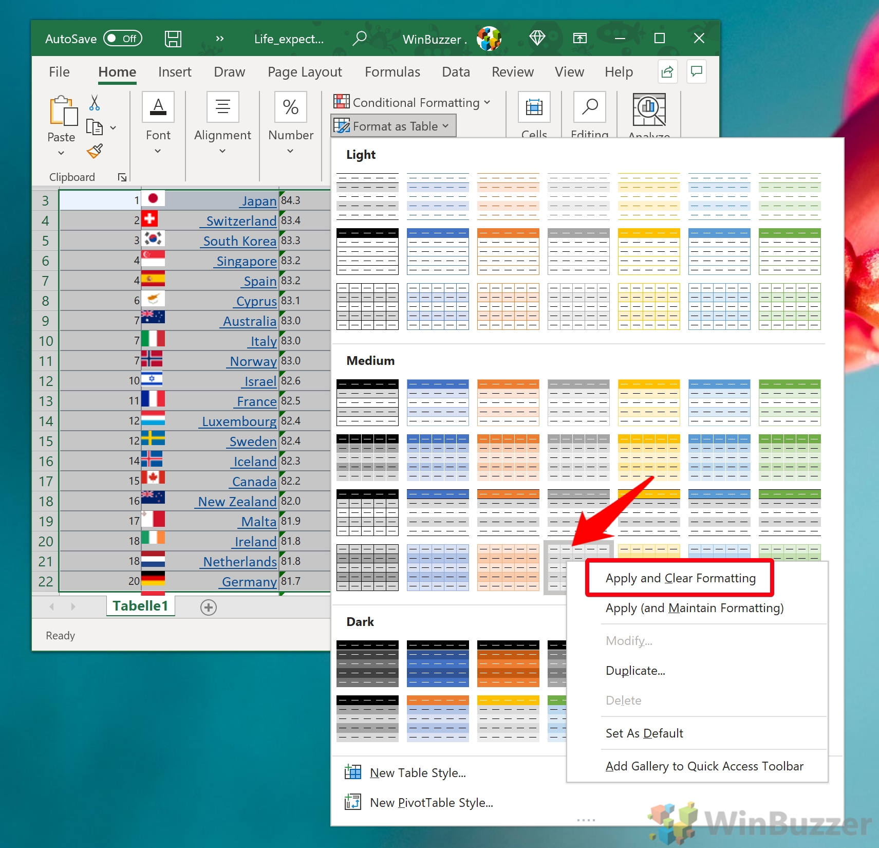
- Choose a Color Scheme
A dropdown menu will appear with various color schemes. Right-click on your desired theme and select “Apply and Clear Formatting” to remove any existing formatting before applying the new table style. Alternatively, choose “Apply (and Maintain Formatting)” to retain your current cell formatting.
- Confirm Table Creation
A “Create Table” prompt will appear. Here, you can adjust the table range if necessary. Make sure to check “My table has headers” if your table includes headers, then press “OK“.

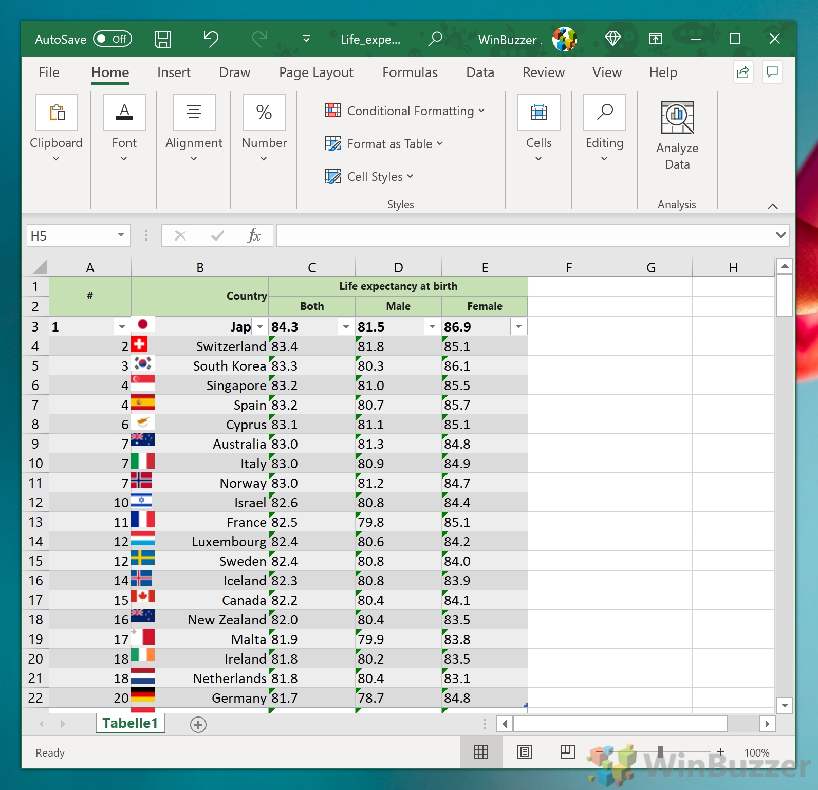
- View Zebra Stripes
Excel will automatically apply the zebra stripes pattern to your table, with alternating row colors for easy reading. This formatting will also apply to any new rows added to the table.
How to Edit Your Zebra Stripes’ Excel Style
If the default color scheme doesn't fit your needs, Excel allows you to customize the zebra stripes by creating a custom table style. As well as selecting a different color from the Quick Styles list, you can add your own custom colors.
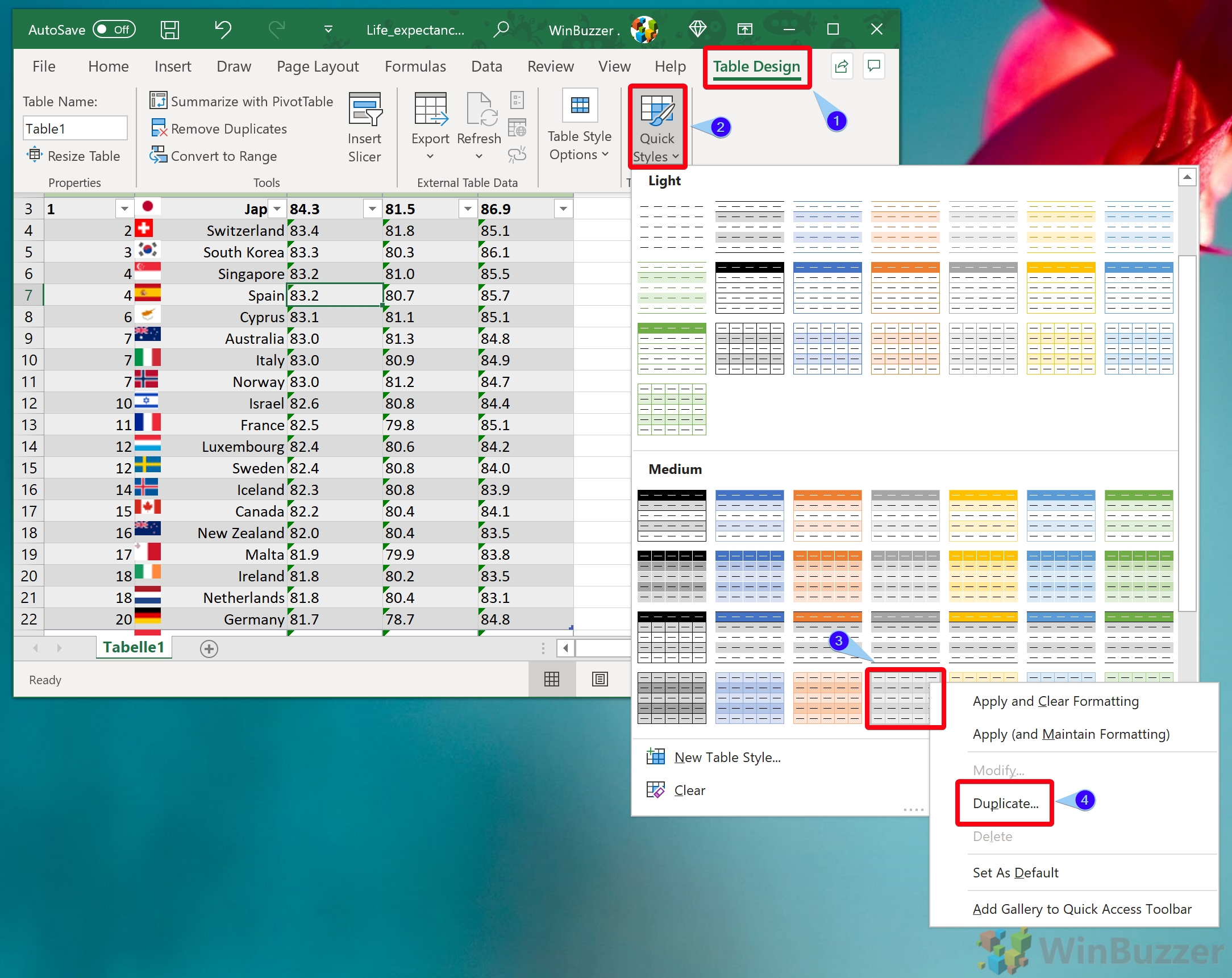
- Duplicate an Existing Style
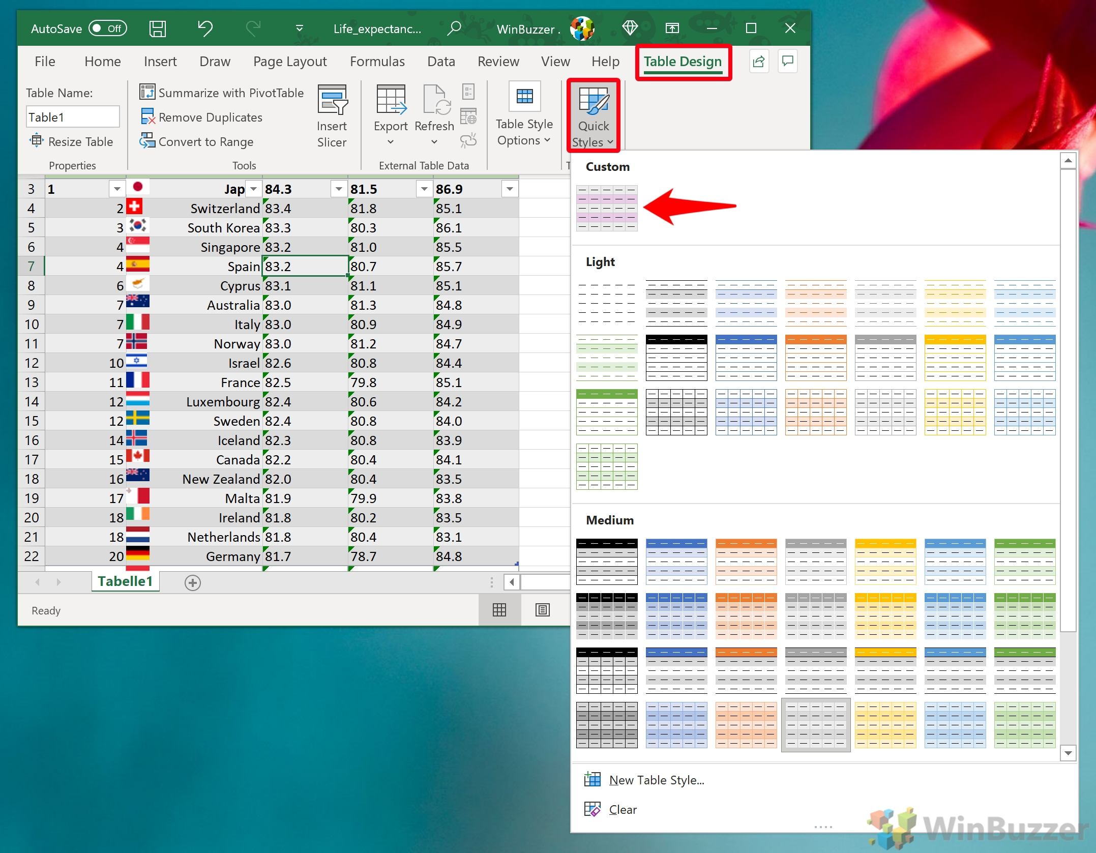
You cannot directly modify the default styles, so you'll need to duplicate one first. Navigate to the “Table Design” tab, click “Quick Styles“, right-click your current style, and select “Duplicate…“.
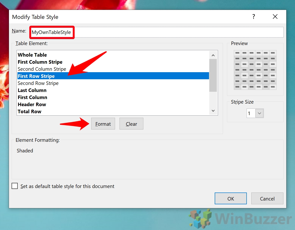
- Name Your Style and Format the First Row Stripe
In the “Modify Table Style” dialog, select “First Row Stripe“. Click the “Format” button to customize the appearance of your alternating rows.
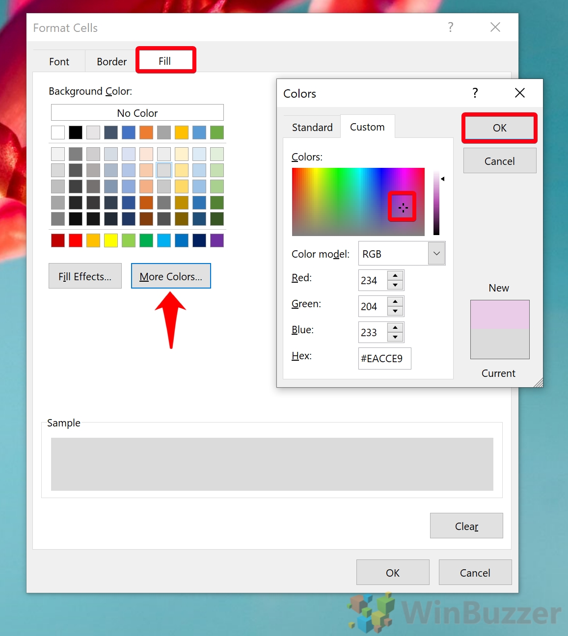
- Select a Color
In the “Format Cells” window, go to the “Fill” tab. Choose a color for your stripes from the preset options or select “More Colors…” to pick a custom shade.
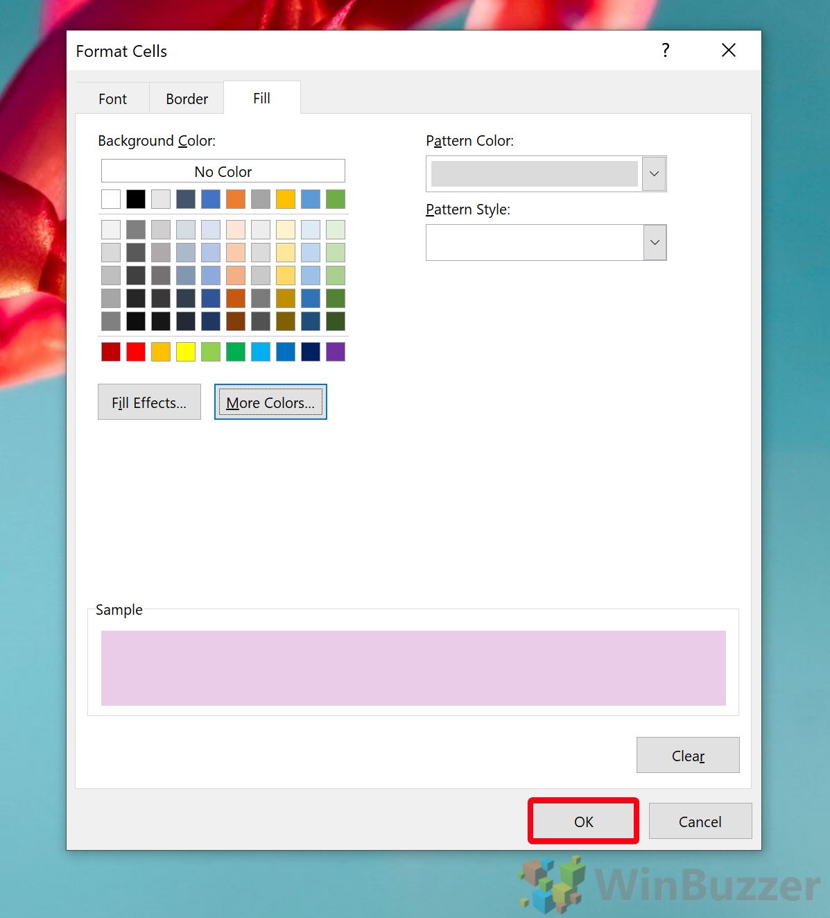
- Apply
After customizing your style, press “OK” to apply the changes.
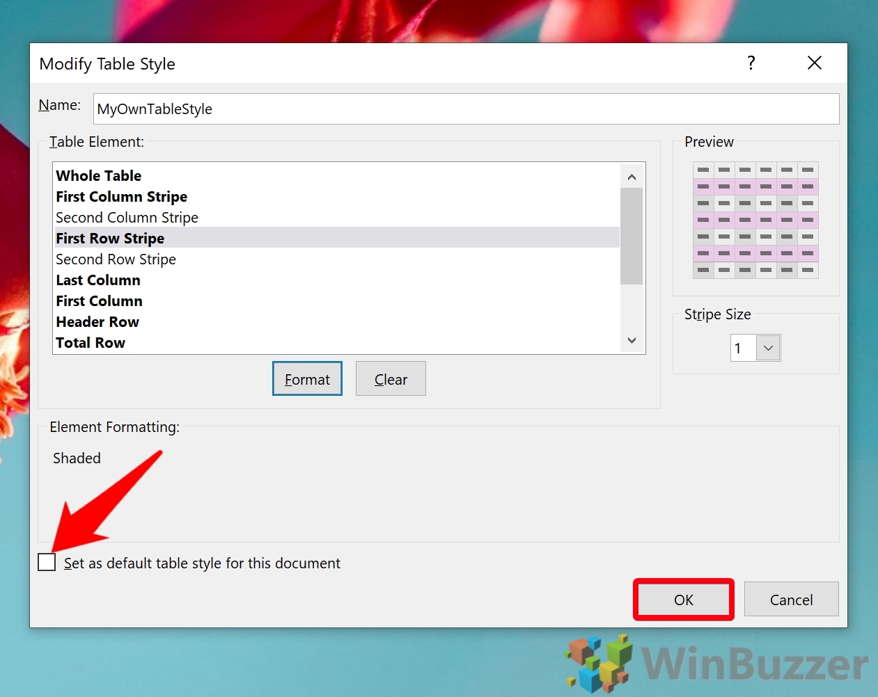
- Select Your Custom Style
To make this style the default for your document, tick “Set as default table style for this document” before clicking “OK” again.
- Select your custom style from the Quick Styles menu
Return to the “Table Design” tab, click “Quick Styles“, and select your newly created custom style to apply it to your table.
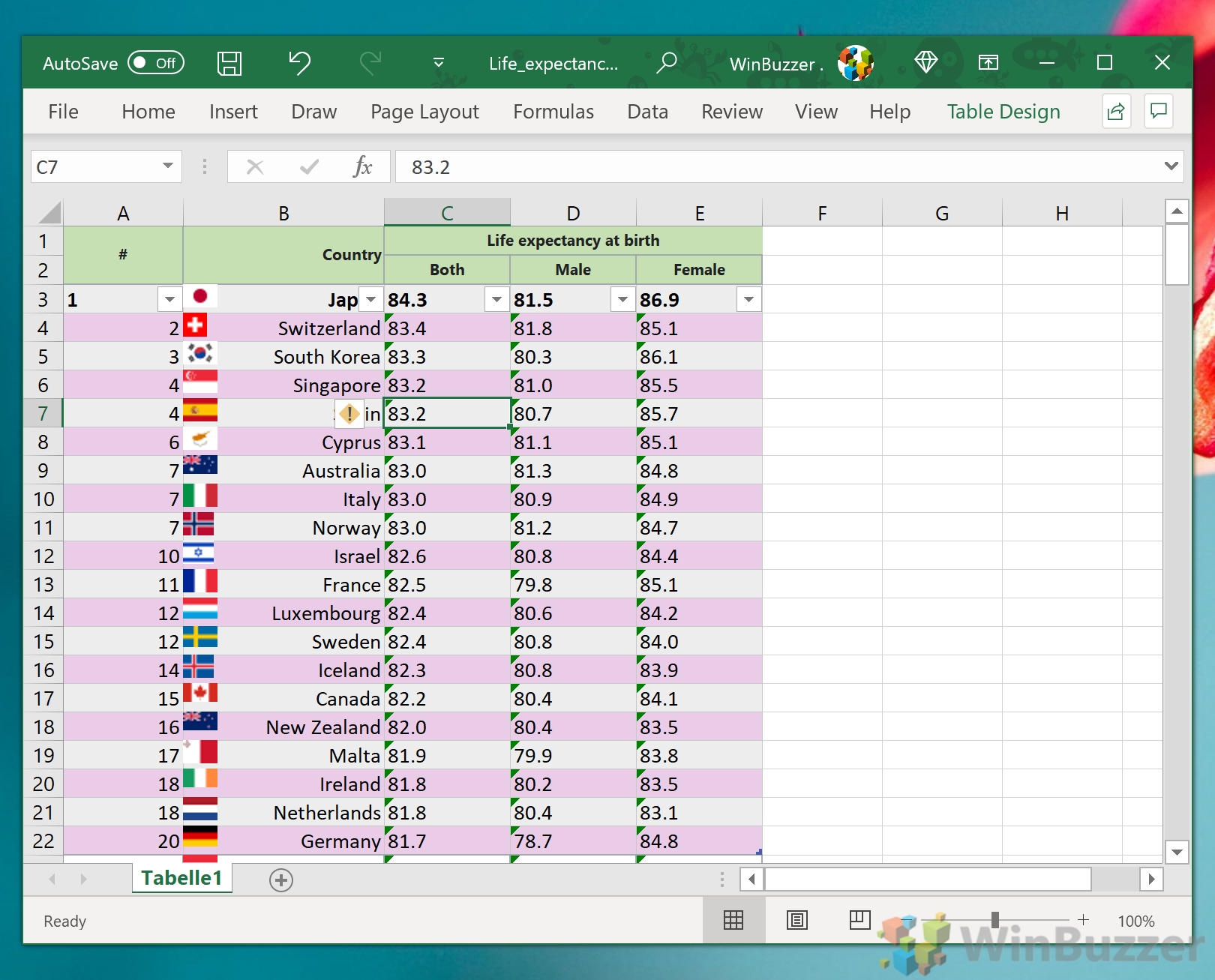
- Enjoy Your Customized Zebra Stripes
Your Excel document will now display the custom zebra stripes style, making your data visually appealing and easier to read.
How to Convert a Table Back into a Range
Generally, it's recommended to keep your Excel data as a table as it allows your to sort, format, and build charts from it more easily. While tables offer numerous benefits for managing data, you might prefer to convert your table back into a regular range but keep the zebra stripes formatting.
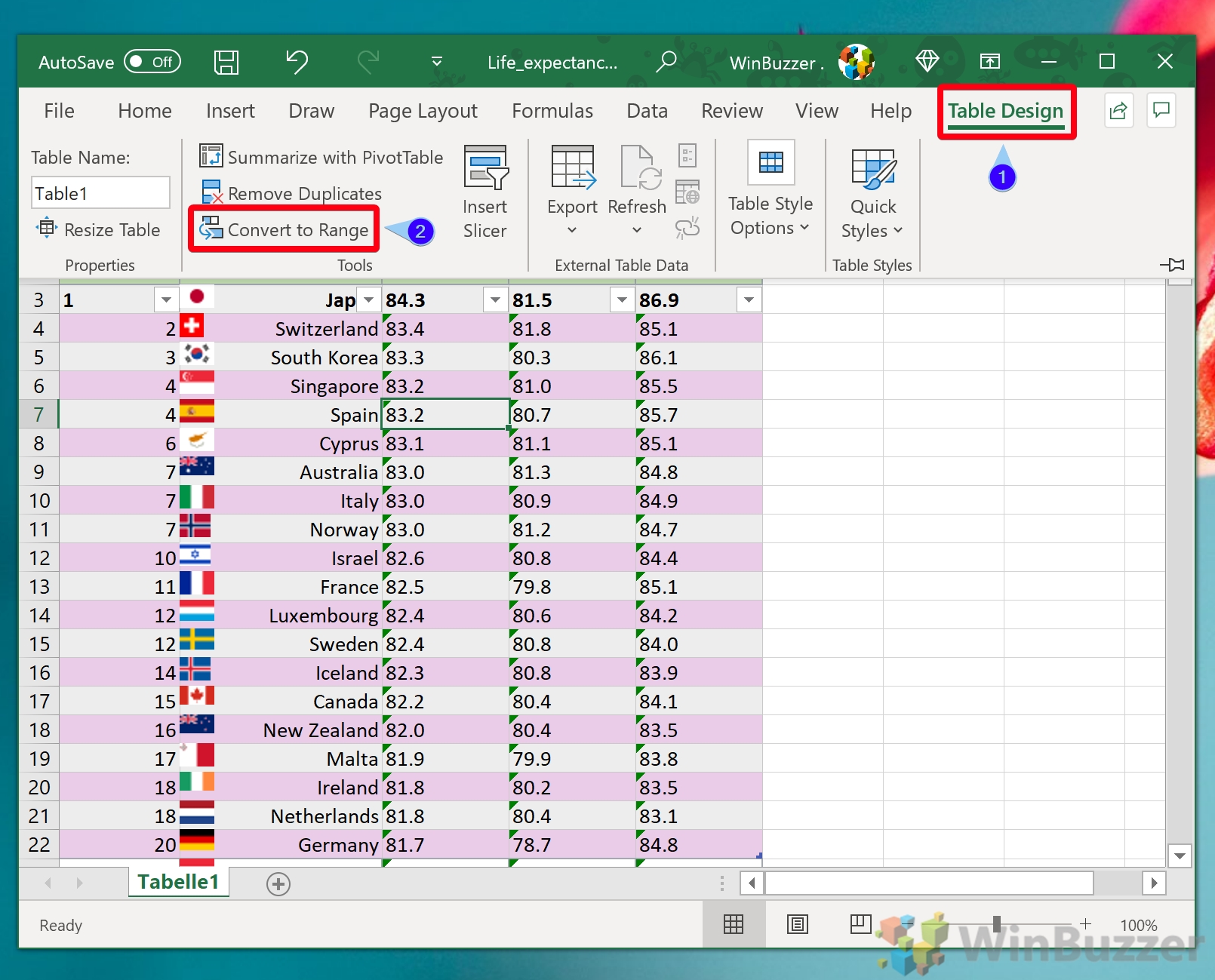
- Initiate Conversion to Range
With your table selected, go to the “Table Design” tab and click “Convert to Range“.
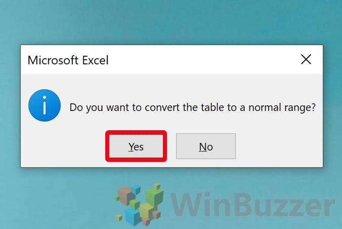
- Confirm Conversion
Excel will prompt you to confirm the conversion. Click “Yes” to proceed. Your table will be converted back into a range, but the banded row formatting will remain intact.
FAQ – Frequently Asked Questions About Excel Zebra Stripes
Can I apply zebra stripes without using the table feature in Excel?
Yes, you can apply zebra stripes manually by using the “Conditional Formatting” feature found under the “Home” tab. First, select the range of rows you want to format. Then, go to “Conditional Formatting” > “New Rule” > “Use a formula to determine which cells to format”. Enter a formula like =MOD(ROW(),2)=0 for every second row, and set the format by specifying the fill color. This method offers flexibility in applying zebra stripes without converting your data into a table format, allowing for customized use cases outside of regular tabular data structures.
Is it possible to apply zebra stripes to columns instead of rows?
Absolutely, although the tutorial focuses on applying zebra stripes to rows, the same principles can be adapted to columns through the “Conditional Formatting” feature. Select the columns you want to stripe, then navigate to “Conditional Formatting” > “New Rule” > “Use a formula to determine which cells to format”. Use a formula like =MOD(COLUMN(),2)=0 to apply formatting to every second column. This can be particularly useful when you wish to visually separate different types of data across columns for improved readability.
How do I ensure zebra stripes are printed correctly in Excel?
To ensure zebra stripes and all content are printed correctly, you should first define the print area by selecting the range to print and going to “Page Layout” > “Print Area” > “Set Print Area”. Then, ensure your print settings are adjusted to include all necessary details by accessing “File” > “Print”. Here you can preview the layout, adjust orientation, and ensure gridlines or headings are included if needed. Adjusting the print quality or choosing a color printer may also be necessary to capture the nuances of the zebra stripes effectively.
Can zebra stripes be dynamic when filtering or sorting data?
Yes, one of the advantages of using tables to apply zebra stripes is that the alternating row color formatting dynamically adjusts when you sort or filter the data within the table. This ensures that the readability improvement offered by the zebra stripes remains intact, regardless of how the data is reorganized, providing a consistent user experience. It's particularly useful in managing large datasets where frequent data manipulation occurs.
Can I save a custom table style for use in other Excel files?
While Excel doesn't include a feature to export and directly apply custom table styles across different files, you can save the file with your custom table style as a template. When starting a new project, open this template file, preserving your custom styles. To create a template, after designing your custom table style, go to “File” > “Save As”, choose “Excel Template (*.xltx)” from the “Save as type” dropdown, and save your file. Opening this template for new projects ensures your custom table style is readily available.
What's the fastest way to apply zebra stripes to multiple tables in a sheet?
For efficiency, after creating your custom table style, you can quickly apply it to multiple tables within the same worksheet by selecting each table individually and choosing your custom style from the “Table Design” tab under “Table Styles”. Holding down the “Shift” key allows you to select multiple tables, or use the “Ctrl” key to select them individually across your worksheet. This method streamlines the application process, especially beneficial in documents containing a significant amount of tabular data.
How do I adjust the thickness of zebra stripes in Excel?
The visual thickness of zebra stripes is directly linked to the row height in Excel. To adjust, right-click the row numbers of the rows you want to modify, and choose “Row Height”. Enter your desired height in the dialog box that appears. This allows you to customize the appearance of your zebra stripes, making them broader or narrower based on your visual preference or the need to accommodate varying amounts of text within the cells.
Are there any limitations to Excel's table feature that might affect zebra stripes?
While Excel's table feature significantly enhances data management and visualization capabilities, including facilitating the implementation of zebra stripes, certain limitations exist. For instance, working with extremely large datasets within a table can impact performance. Additionally, while tables support structured references that simplify formula creation, some complex data analysis tasks might require the data to be outside a table format. Consider your project's needs to decide whether to use tables or direct formatting for zebra stripes.
Can I change the order or pattern of zebra stripes?
The default zebra striping pattern in Excel is an alternating row color scheme. For a custom pattern, such as two dark rows followed by a light row, manual formatting or advanced “Conditional Formatting” techniques are required. For instance, you can use a formula in conditional formatting like =MOD(ROW(),3)=1 or =MOD(ROW(),3)=2 for creating customized patterns, providing you the flexibility to design a visually distinct pattern that meets your specific needs.
How do I apply zebra stripes to only specific rows or conditions?
For applying zebra stripes based on specific conditions, “Conditional Formatting” offers the most flexibility. For example, to stripe only rows where a certain cell contains a specific value, select your range and use a formula like =AND(MOD(ROW(),2)=0, $A1=”Specific Value”) in the conditional formatting rule. This approach allows you to combine the visual benefits of zebra stripes with logical conditions, tailoring the data presentation to highlight particular aspects of your dataset dynamically.
Is it possible to automatically extend zebra stripes formatting to new rows?
By applying zebra stripes through Excel's table feature, any new rows added to the bottom of the table will automatically inherit the same formatting, including the alternating row colors. This automation is beneficial for maintaining consistent data presentation as your table grows, reducing the need for manual updates to the formatting.
How do zebra stripes affect cell readability in printed documents?
Zebra stripes can significantly enhance the readability of printed documents by visually separating rows. When preparing to print, choose lighter shades for your stripes to ensure that the text remains legible. Utilize print preview to adjust settings as needed and consider the paper quality and printer capabilities, as these factors can affect the final output quality including how well the zebra stripes are reproduced.
Can the color of zebra stripes be dynamically changed based on cell values?
Although not directly related to zebra striping, “Conditional Formatting” allows for the dynamic changing of cell or row colors based on cell values. By setting rules that connect cell values to specific colors, you can create an evolving visual landscape within your spreadsheet that reflects data trends or highlights critical data points, adding another layer of data analysis to the visual representation.
What are the best practices for using zebra stripes in shared or collaborative Excel files?
When sharing Excel files that utilize zebra stripes, especially in collaborative environments, ensure that all collaborators understand the method used (table format vs. conditional formatting). Document any customizations and choose color schemes that are accessible to individuals with color vision deficiencies. Clarity, consistency, and accessibility should guide your decisions, ensuring that the formatted spreadsheet remains functional and visually effective for all users.
How can I remove zebra stripes formatting from my Excel sheet?
If you've applied zebra stripes by converting your data into a table, first convert the table back to a range by selecting any cell within the table, going to the “Table Design” tab, and choosing “Convert to Range”. Confirm the action when prompted. Then, remove any residual formatting by selecting the affected cells, navigating to the “Home” tab, and using “Clear” > “Clear Formats”. This sequence of actions effectively removes both the table structure and any associated zebra stripe formatting, returning your data to its original unformatted state.
Related: How to Hide and Unhide Rows and Columns in Excel
The ability to hide and unhide rows and columns in Excel is particularly useful for managing large datasets, protecting sensitive information, and maintaining a clean, focused workspace. Our other tutorial shows you how to hide and unhide rows and columns in Excel, ensuring that you can control the visibility of your data with ease.

Related: How to Remove Spaces in Excel
When managing extensive datasets in Excel, ensuring data consistency is crucial. An all too common inconsistency is unwanted spaces — whether they creep in at the beginning or end of a text string, appear as unwarranted gaps between words, or are unintentional space characters throughout your content. In our other guide, we show how to use the Replace Feature, the TRIM funcion, and the SUBSTITUTE function to seamlessly eliminate unwanted spaces in Excel.
Related: How to Make a Graph in Excel (Bar Chart, Pie Chart, Etc.)
Excel's dedicated graphing tools allow you to quickly switch between a variety of chart types and customize them once you've chosen. In our other guide, we show you how to make a graph in Excel, then customize the chart's colors, title, style, label, and more.

Related: How to Autofit Rows and Columns in Excel
By default, Excel cells are not very wide. You can fit a total of eight full characters, which is enough for many numbers, but not much for text. In our other guide, we show you how to autofit in Excel for both columns and rows, using double-click. shortcuts, and the ribbon.