One of the most common types of sorting in Excel is alphabetical sorting. Whether it’s a list of names, businesses, or mail addresses, sorting helps to organize and keep track of what you’re doing. Today we’re going to help you with that by showing you how to alphabetize in Excel for both rows and columns.
While there are several ways to alphabetize in Excel, the most consistent is the sorting feature in the Data section of your ribbon. We’ll show this feature and as well the A to Z filter shortcut.
How to Sort Columns Alphabetically in Excel
This method allows organizing column data in alphabetical order, utilizing Excel’s built-in sorting features. It´s ideal for when you have lists or databases in Excel and need to quickly find or organize information, sorting columns alphabetically can enhance data readability and accessibility. Whether you’re dealing with names, locations, or any other text-based data, this approach ensures that your data is systematically arranged from A to Z, making it easier to navigate and analyze.
-
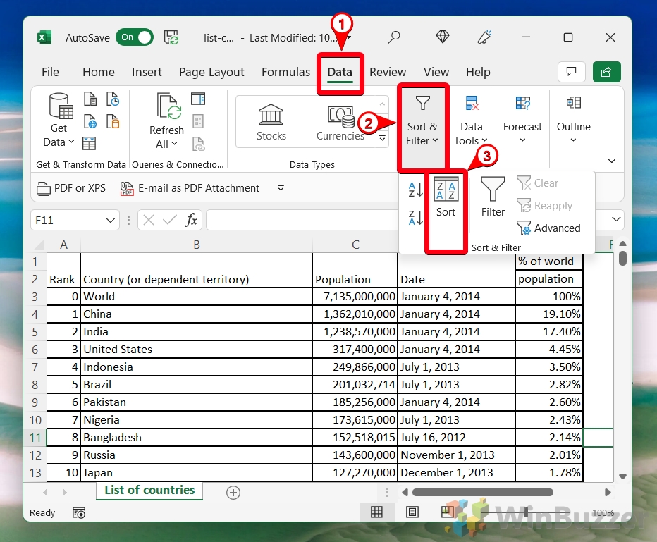
Open the “Data” tab and select “Sort & Filter > Sort”
Navigate to the Data tab on Excel’s ribbon. Here, you’ll find the sorting features. Look for “Sort & Filter” and click on “Sort” to begin organizing your column data alphabetically.

-
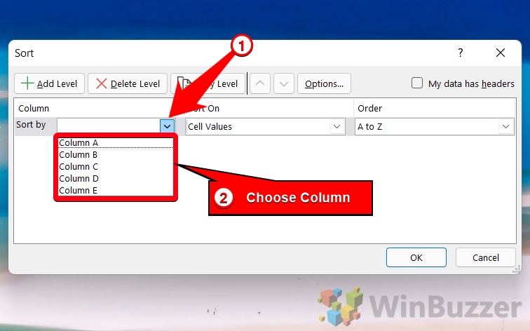
Choose your column in the “Sort by” dropdown
In the sorting dialog box that appears, you’ll see a “Sort by” dropdown menu. Click on this dropdown and select the column you wish to alphabetize. This tells Excel specifically which data column you’re looking to organize.

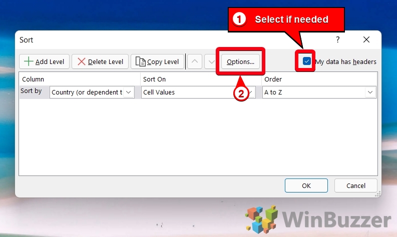
- Set the sorting options
If your data includes headers, make sure to check the “My data has headers” box to avoid sorting your headers as regular data. Then, set the sorting order. For alphabetical organization, choose “A to Z” from the order dropdown. This will sort your column data starting with the letter A at the top. Of course, you can also change this to Z to A or a custom list type if you wish. Just press “OK” when you’re done.
- Check sorting results
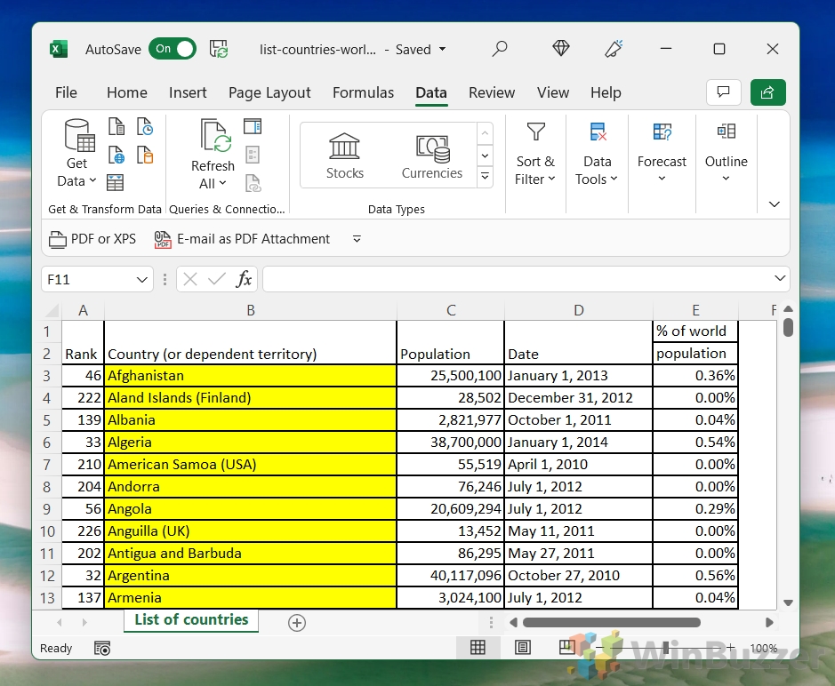
Once you’ve set your sorting preferences, click “OK” to apply them. Excel will automatically reorganize your selected column data in alphabetical order. Review your column to ensure everything is sorted as expected.
How to Alphabetize a Column in Excel
Alphabetizing a column specifically focuses on rearranging the data within a single column, maintaining the relational integrity of each row’s data. This method is particularly useful when you need to sort individual columns without altering the overall structure of your table or dataset. It’s applicable in scenarios where only one aspect of your data requires organization, such as sorting a list of names in a guest list, without affecting associated data like email addresses or phone numbers.
- Access “Sort & Filter > Sort” in the “Data” tab
Start by going to the Data tab. Click on “Sort & Filter” and then “Sort” to open the sorting dialog box.
-
Enable “My data has headers” and open “Sort Options…”
If your rows include header information, ensure “My data has headers” is checked to keep your headers intact. Then, click on “Options…” to access more sorting settings tailored for rows.

-
Switch to “Sort left to right” and confirm
In the Sort Options dialog, you’ll find the ability to change the sorting orientation. Select “Sort left to right” to indicate you’re organizing rows, not columns. Confirm your choice by clicking “OK“.

-
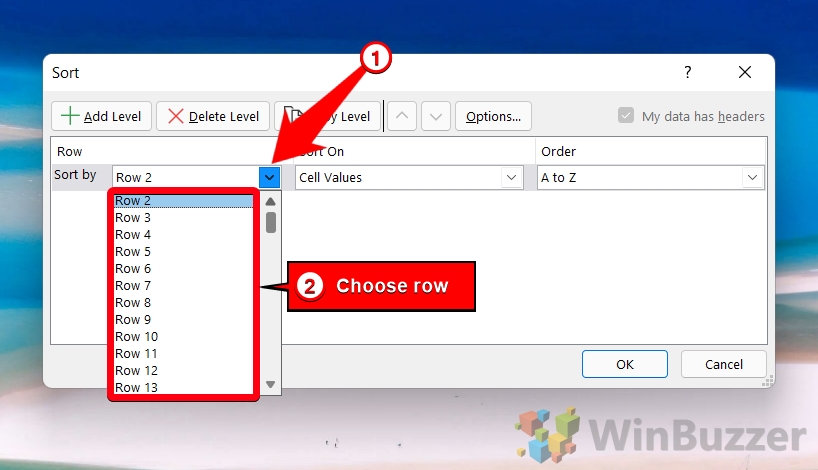
Change the “Sort by” dropdown to your desired row
Back in the main sorting dialog, use the “Sort by” dropdown to select the row you’re alphabetizing. This step defines which row’s data Excel will use as the basis for the alphabetical sorting.

- Set the sorting order and apply
Finally, choose “A to Z” from the Order dropdown to sort your data alphabetically from left to right. Apply your settings by clicking “OK“, and Excel will rearrange your selected row accordingly. Excel will instantly alphabetize your row to match your preference. You can, of course, sort from Z to A instead if you wish.
How to Alphabetize in Excel Using Shortcuts
This more efficient way to alphabetize data in Excel is ideal for smaller datasets or when you need to make quick adjustments. By using keyboard shortcuts and quick-access toolbar options, you can streamline the sorting process, saving time and effort. This method is perfect if you are looking to increase productivity and efficiency in data management tasks, allowing for rapid reordering of information with just a few clicks.
-
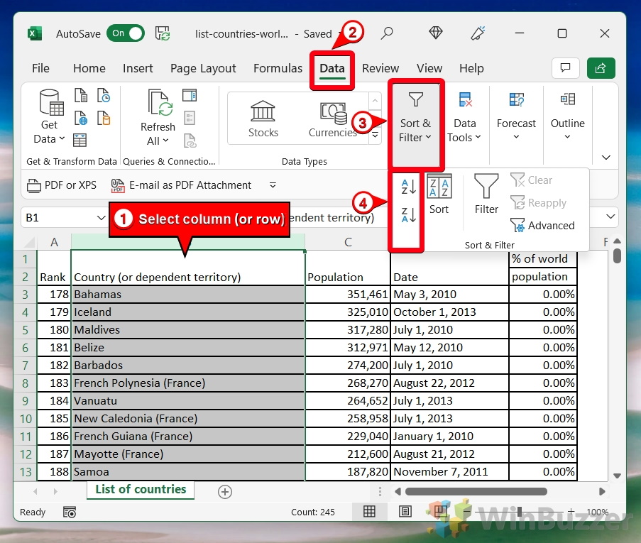
Select the column, open the “Data” tab of the ribbon, and click “Sort & Filter > AZ / ZA”
Select the data you want to sort. Then, in the Data tab, find “Sort & Filter“. Here, you’ll see the “AZ” (ascending order) and “ZA” (descending order) buttons. Choose “AZ” for alphabetical sorting. You can select a column or row by clicking on its letter or number in the sheet border.

-
Tick “Continue with the current selection” and press “Sort”
If prompted, ensure “Continue with the current selection” is selected and click “Sort“. This confirms your selection and initiates the sorting process.

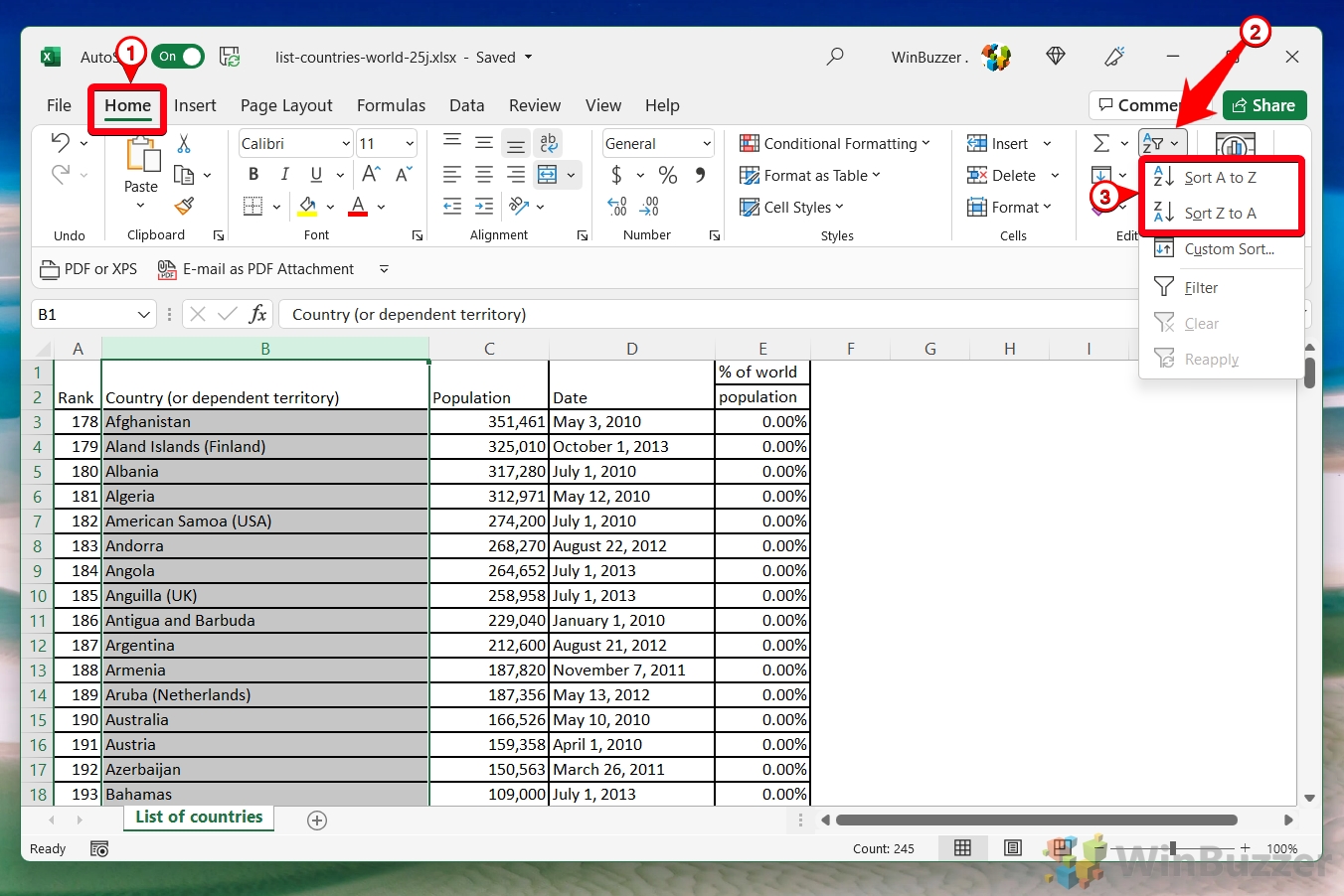
- Alternatively, use the “Home” tab sorting options
Another quick way to sort is via the Home tab. Here, in the Editing section, you’ll find similar “Sort A to Z” and “Sort Z to A” buttons for immediate data organization.
FAQ – Frequently Asked Questions About Sorting in Excel
Why won’t Excel sort my data alphabetically?
Sorting issues in Excel can stem from a variety of sources. Firstly, ensure no leading spaces are present, as Excel might interpret a space as the first character, affecting the sort order. Secondly, verify the consistency of your data types; mixed data types (text and numbers) in a single column can lead to unexpected sorting results. Lastly, examine your range for merged cells, which can complicate the sorting process. To resolve, consider unmerging cells or sorting data before merging.
How do I sort columns in Excel without affecting other data?
To ensure that sorting a column doesn’t disrupt other data, it’s crucial to treat your data as a single block or table. Highlight the entire range of data you wish to sort, or convert your range into a table by selecting it and using the Insert > Table option. When sorting, always use the Data > Sort feature, and ensure the “My data has headers” option is checked to keep your headers fixed and to sort data rows in relation to each other.
What are the advanced sorting options in Excel?
Beyond basic alphabetical and numerical sorting, Excel offers advanced options like sorting by cell color, font color, or conditional formatting icons. To access these, in the Sort dialog box, select a column to sort by, then choose “Cell Color,” “Font Color,” or “Conditional Formatting Icon” in the “Sort On” dropdown. You can prioritize the sorting based on color or icon order, which is particularly useful in visually categorized data sets.
How do I keep rows together when sorting in Excel?
When sorting by columns, Excel keeps row data together by default. However, it’s crucial to select the entire dataset or table before sorting to ensure that all related data in a row stays together. If you’re sorting a table, Excel will treat the table as an entity, keeping rows intact. For a range, drag to select the entire range or click the column header to select the entire column, then proceed to sort.
Can I sort columns independently in Excel?
Sorting columns independently can disrupt the relational integrity of your dataset. However, if necessary, you can select a single column (excluding the header) and use the “Sort A to Z” or “Sort Z to A” buttons under the Data tab. Be mindful that this action will sort the selected column’s cells independently of the rest of your data, potentially scrambling the relationship between rows.
Why does Excel sort numbers incorrectly sometimes (e.g., 10 before 2)?
This issue often arises when numbers are formatted or stored as text, leading Excel to sort them alphabetically (‘1’ comes before ‘2’, hence ’10’ before ‘2’). To correct this, convert the text-formatted numbers to actual numbers. You can do this by selecting the column, going to the Data tab, and choosing Text to Columns > Finish. Ensure the column’s format is set to Number by right-clicking the column header, choosing Format Cells, and selecting Number.
How do I create a custom sort list in Excel?
To create a custom sort list, navigate to File > Options > Advanced, and scroll down to the General section to find Edit Custom Lists. In the Custom Lists dialog, you can either type a new list or import one from an existing range in your worksheet. Once created, these lists can be used in the Sort dialog by choosing “Custom List…” in the Order dropdown, allowing for sorting based on user-defined criteria.
How do I sort by date and keep rows together in Excel?
Sorting by date follows the same principles as sorting alphabetically. Ensure your dates are formatted correctly (check by right-clicking the cells, selecting Format Cells, and verifying that they’re set under a Date format). Select your dataset, then use the Sort feature in the Data tab, choosing your date column in the “Sort by” dropdown. Excel will recognize the date format and sort accordingly, keeping row data together.
Can Excel sort data horizontally?
To sort data horizontally, access the Sort dialog, click on Options, and choose “Sort left to right“. Then, in the “Sort by” dropdown, select the row that you wish to use as your sorting basis. This feature is particularly useful for datasets where the relational data is aligned horizontally rather than in the traditional vertical column layout.
How do I sort alphabetically with multiple columns and rows in Excel?
For multi-level sorting, use the “Custom Sort” option from the Sort dialog. Here, you can add levels to sort by one column and then another. For example, you might first sort by Last Name and then by First Name to organize data alphabetically by last name, and then within each last name group, by first name. This is achieved by adding a level for each column you wish to sort by and defining the order for each.
How do I sort only one column in Excel without affecting others?
To sort a single column without altering adjacent columns, select the cells in the column (excluding the header), right-click, and choose “Sort > Sort A to Z” or “Sort Z to A“. Be cautious, as this method disrupts the original relationship between the column’s data and the rest of your table, which might not be desirable in most cases.
What is the quickest way to rearrange column order in Excel?
For manual rearrangement of columns, simply select the entire column by clicking its header, then drag and drop it to the desired location. A green guide line will appear, indicating where the column will be placed upon release. This method is effective for quickly reorganizing columns without sorting the data they contain.
How do I rearrange columns in Excel?
To rearrange columns, click on the column header to select the entire column, then drag it to the new position. A thick green line will indicate where the column will be placed when you release the mouse button. Ensure that “Cut, Copy, and Sort inserted objects with their parent cells” is enabled in Excel’s advanced options to maintain data integrity during the move.
How do I sort multiple columns in Excel without mixing data?
To sort multiple columns while keeping related data together, use the “Custom Sort” feature by selecting your data range, clicking on Sort, and then on “Custom Sort“. Add levels to specify the columns and sort orders. For instance, you might sort by “Department” and within each department, sort by “Employee Name”. This maintains data integrity across rows while sorting based on multiple columns.
How do I manually sort columns?
For manual sorting, select the column or columns by clicking their headers, cut them using Ctrl+X, and paste them into the desired location using Ctrl+V. For non-contiguous columns, repeat the cut and paste process for each. This method allows for precise control over column order but should be used with caution to preserve data relationships.
Related: How to Structure Collected Data in Excel
Excel is a powerful tool for collecting, analyzing and presenting data. However, to make the most of Excel’s features, you need to structure your data properly. In our other guide, we show you how to structure collected data in Excel using some best practices and tips.

Related: How to Change the Date Format in Excel
Dates and times are not just mere values in Excel – they are crucial data points that drive analytics, reporting, and day-to-day data entry. Excel acknowledges this by providing a plethora of options to format and customize these values. In our other guide, we show you
how to change the date format in Excel to other local formats and using a custom format.

Related: How to Freeze a Row or Column in Excel
Excel’s freeze pane feature is an invaluable tool for navigating large datasets without losing sight of your reference points. Whether you’re working with financial reports, data analysis, or any extensive spreadsheet, the ability to lock specific rows or columns in place as you scroll through your data can drastically enhance your productivity and data interpretation accuracy. In our other guide, we show you multiple ways to freeze and lock the rows and columns in an Excel sheet using the ribbon interface.

Last Updated on April 22, 2024 12:40 pm CEST by Markus Kasanmascheff


