Creating a drop down list in Excel is an essential skill for anyone who regularly works with spreadsheets. This feature enhances data entry efficiency, ensures consistency, and minimizes errors, making it invaluable in various applications such as data analysis, financial reporting, and inventory management.
How Drop Down Lists in Excel Work
At its core, a drop down list in Excel is a user interface tool that confines user input to a specific set of values. This is particularly useful in scenarios where input needs to be standardized, such as in forms, surveys, or financial models. By presenting a predefined list of choices, it ensures that data entered into the spreadsheet is uniform and accurate.
Drop Down Lists and Data Validation
The drop down list feature in Excel is part of a broader set of tools known as Data Validation. Data Validation is crucial for maintaining the integrity of the data in your spreadsheets. It not only helps in creating drop down lists but also in setting up rules for what kind of data can be entered into a cell. For instance, you can restrict a cell to only accept numerical values, dates, or a specific text length. This feature is incredibly useful for preventing errors in data entry and for ensuring that the data collected through your Excel sheets adheres to certain standards.
Advanced Uses of Excel Drop Down Lists
Beyond basic data entry, drop down lists can be used for more advanced purposes. For instance, they can be combined with other Excel functions to create dynamic and interactive reports. You can also use them to control the input for more complex formulas, thereby increasing the interactivity and functionality of your Excel models.
How to Add a Drop Down List in Excel via Data-Validation
Data Validation is a powerful feature in Excel that ensures the data entered into a cell adheres to specific criteria. By utilizing this tool, you can create a drop down list that restricts user input to a pre-defined set of options. This method is particularly useful for standardizing data entry and ensuring accuracy in scenarios where only certain inputs are valid. For example, you might use it to limit responses in a survey, to categorize items in an inventory list, or to control input in a financial model. This approach is ideal for both beginners and advanced users seeking to maintain consistency and reliability in their data.
- Create a list of items for the drop down list
You need to have a list of items you want to include in your drop down menu. These items can be typed in a column or a row in the same worksheet where you want the drop down list, or on a different sheet.

- Select the Cell for the Drop Down List
Click on the cell where you want the drop down list to appear and open the “Data” tab. To hide this list from the main table area you can use an empty column on the right or place it on a different Excel sheet.

- Open the Data Validation Dialog Box
Click on “Data Validation” in the “Data Tools” group. This opens the Data Validation dialog box.

- Select “List” in “Validation criteria”
In the Data Validation dialog box, under the “Settings” tab, you will find an option labeled “Allow”. Click on it and select “List” from the dropdown menu. If your list is in cells B2 through A10, you would enter “=$A$1:$A$10”.

- Check “In-cell dropdown” and “Ignore blank” to allow non-selection
“In-cell dropdown” enables the actual drop down list in the cell. This means that when you click on the cell, you will see a small arrow on the right side of the cell, indicating that there is a drop down list from which you can select values.
“Ignore blank” allows users to leave the cell empty without causing a validation error. This is useful when the input in the cell is optional, and you don't want to force users to make a selection from the drop down list.

- Click on “Source” to select the range of drop down list items

- Select the drop-down item-list
If your list is on the same worksheet, you can simply select the range using your mouse or type the range in manually. if your list is in cells A1 through B11, you would enter “=$B$2:$B$11”.
If the list is on a different sheet, you need to include the sheet name, e.g. “=Sheet2!$B$2:$B$11”.

How to Set Properties for a Drop Down List in Excel
Once a drop-down list is created in Excel, the next important step is setting its properties to optimize its functionality and to customize the behavior and appearance of the drop-down list to fit specific needs. Here we show how to modify properties such as allowing or disallowing blank entries, setting up input messages to guide users, and defining error messages to display when invalid data is entered.
These settings are crucial for enhancing the user experience and ensuring data integrity. Tailoring these properties makes the drop-down list more interactive and user-friendly, particularly in environments where multiple individuals with varying levels of Excel proficiency use the spreadsheet.
- Switch to “Input Message” and “Check “Show input message when cell is selected”

- Enter the input message
This message will appear when the cell is selected, guiding users on what to do. Fill in the “Title” and “Input message” fields with your desired text.

- Switch to “Error Alert” and select “Show error alert after invalid data is entered”
This creates a custom error message that will appear if someone enters a value that's not in the drop-down list.

- Select the type of error alert you want to use
Stop: When a user enters invalid data, a Stop message box appears, featuring a red ‘X' icon. This style prevents the user from leaving the cell until they enter a valid value or undo their entry. It's useful when you must ensure that only valid data is entered and you can't allow any exceptions.
Warning: When a user enters invalid data, the Warning message box appears with options to ‘Yes', ‘No', or ‘Cancel'. Choosing ‘Yes' allows the user to override the validation rule and keep the invalid data. ‘No' returns the user to the cell to correct the entry, and ‘Cancel' undoes the entry. This style is useful when you want to strongly discourage invalid entries but still allow users the flexibility to override the rule if necessary.
Information: When invalid data is entered, the Information message box appears with ‘OK' and ‘Cancel' options. ‘OK' allows the user to leave the cell with the invalid entry, while ‘Cancel' returns them to the cell to make a correction. This style is appropriate when you want to gently remind users of the validation rule but are fine with them ignoring it.

- Choose “Title” and the “Error message”

- Save with “OK”

How to Use a Drop Down List in Excel
Once set up, users can click and select the defined items from the drop-down list.
- Hovering over the cell shows the “Input Message”
A click on the arrow button shows the available list items.

- Items of the drop down list can be selected with a click to use them in the respective cell

How to Edit a Drop Down List in Excel
Editing a drop down list is easy and consists of two steps.
- Locate the list of items in the list: Select the cell where the drop-down list appears, open the “Data Validation” dialog box as described in method 1 and check the “Source” field where the range of cells with the items is shown.
- Edit the Excel drop down list items: Jump to the range of cells with the drop-down list items and edit it there.
- Add item to drop down list in Excel: You can add additional items to the Excel drop-down list by extending the item list and adjusting the “Source” in the “Data Validation” dialog box.
FAQ – Frequently Asked Questions About Excel Drop-Down Lists
Can I use formulas in the source list for a drop-down in Excel?
Absolutely. You can dynamically generate your source list for a drop-down menu using formulas such as CONCATENATE, IF, or even VLOOKUP. Place these formulas in the cells that you designate as your source list. Excel's Data Validation will then reference these cells to populate the drop-down list. For instance, if you're using an IF formula to display certain items under specific conditions, your drop-down list will update automatically based on the formula's output.
How can I make a drop-down list's selections influence other cells' formulas in Excel?
The selection from a drop-down list can be incorporated into formulas to create dynamic and responsive Excel models. For example, if your drop-down list is in cell A1, and you want to perform a calculation in cell B1 based on the selection, you can use a formula like =IF(A1=”Option 1″, B1*10, B1*20). This formula will perform different calculations in B1 depending on the selection made in A1, effectively making your spreadsheet interactive and adaptable to user input.
Is it possible to link a drop-down list to a cell's comment in Excel?
While Excel does not provide a direct feature to link drop-down list selections to comments, you can achieve this functionality using a simple VBA script. The script can monitor changes in the cell containing the drop-down list and update the comment accordingly. This requires basic knowledge of VBA and the use of the Worksheet_Change event to trigger the comment update.
Can I set a default value for a drop-down list in Excel?
To set a default value for a drop-down list, simply enter the desired default value in the cell before applying the drop-down list. When the workbook is opened or the sheet is activated, this value will appear as the default selection. If you need the default value to reset every time the sheet is activated or under certain conditions, you can use a VBA script to automate this process.
How do I create a drop-down list that automatically updates based on another sheet's changes in Excel?
For a drop-down list that updates automatically when changes are made on another sheet, use a dynamic named range. This can be achieved by defining a named range using the OFFSET and COUNTA functions to create a range that automatically adjusts to include new data. For example, if you have a list in Sheet2 starting from A1, you can create a named range with the formula =OFFSET(Sheet2!$A$1,0,0,COUNTA(Sheet2!$A:$A),1). This named range will expand or contract based on the entries in Sheet2 and can be used as the source for your drop-down list.
How can I use drop-down list selections to trigger macros in Excel?
To trigger macros based on drop-down list selections, you can use the Worksheet_Change event in VBA. This event will run a macro whenever a change is made in the worksheet. You can include a condition within this event to check if the change was made in the cell with the drop-down list and then execute a specific macro based on the selected value. This requires some VBA programming knowledge to set up but can greatly enhance the interactivity of your Excel workbook.
Is it possible to have conditional formatting in a drop-down list that changes the text color based on selection in Excel?
While the text within a drop-down list cannot be formatted directly, you can apply conditional formatting to the cell containing the drop-down list to change its appearance based on the selected value. For example, you can set up rules that change the cell's background color or text color when certain options are selected. This is done by selecting the cell, going to the Conditional Formatting menu, and setting up new rules based on the cell's value.
Can a drop-down list in Excel reference a list in another workbook?
Referencing a list in another workbook for a drop-down list is possible but comes with limitations. Both workbooks need to be open for the drop-down to function correctly. The source reference should include the full path of the workbook, the sheet name, and the cell range. However, this setup can be fragile and might lead to errors if the source workbook is not open or the path changes.
How can I export or import drop-down lists between Excel files?
To export or import drop-down lists, you can simply copy the cell containing the drop-down list from one Excel file and paste it into another. Ensure that the source data for the drop-down list is also copied or available in the target workbook. If the list relies on a named range or a specific sheet structure, these elements must be replicated in the new workbook for the drop-down to function correctly.
What's the difference between using a named range and direct cell references for drop-down lists in Excel?
Using a named range for your drop-down list offers greater flexibility and clarity, especially for dynamic lists that might change in size. Named ranges can automatically adjust to include new data if set up with dynamic formulas like OFFSET. Direct cell references are simpler and more straightforward but need to be manually adjusted if the size of your list changes. Named ranges also make your formulas and data validations easier to read and maintain.
How do I align text within a drop-down list in Excel?
The alignment of text within a drop-down list in Excel is controlled by the cell's alignment settings. To change the text alignment, select the cell containing the drop-down list and adjust the alignment options under the Home tab. The text in the drop-down will align according to the cell's horizontal and vertical alignment settings.
Can I format numbers or dates within a drop-down list in Excel?
Formatting for numbers or dates within a drop-down list is derived from the source cells. To display formatted numbers or dates in your drop-down list, apply the desired number or date format to the cells in your source list. The drop-down will then display the values in the formatted style.
Is it possible to control the width of a drop-down list in Excel?
The width of the drop-down list in Excel is automatically determined by the width of the widest entry in the list. There is no direct way to manually adjust the width of the drop-down. If the list entries are too wide, consider abbreviating them or increasing the column width where the drop-down list is located to accommodate longer entries.
Can I use data validation to create a drop-down list that references a table column in Excel?
Yes, data validation can be used to create a drop-down list that references a column in an Excel table. This is particularly useful because table columns automatically adjust when new items are added or removed, keeping your drop-down list up to date. Simply use the table column reference (e.g., TableName[ColumnName]) as the source in your Data Validation settings.
How do I make a drop-down list visible at all times in Excel, not just when clicking on the cell?
To have a drop-down list or a similar control visible at all times, you can use an ActiveX Combo Box or a Form Control Combo Box instead of the standard Data Validation drop-down. These controls are available from the Developer tab under “Insert” and can be configured to display a list of items. They remain visible on the sheet and provide a more interactive element for users.
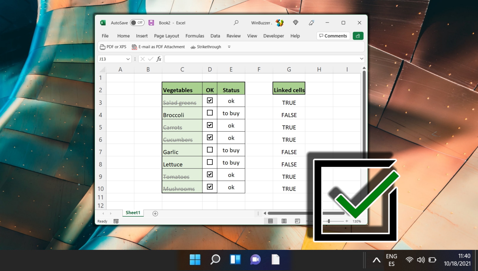
Extra: How to Insert a Checkbox in Excel
A checkbox is a simple control that I'm sure everybody will have encountered online, often as part of a cookie dialog or where you'll tell a site to remember you being logged in. Checkboxes in Excel are much the same thing, but you may not be aware of how useful they can be. In our other guide, we show you how to add check boxes in Excel, demonstrate how they function as part of a spreadsheet, and show how they can be used to build a To-Do list.
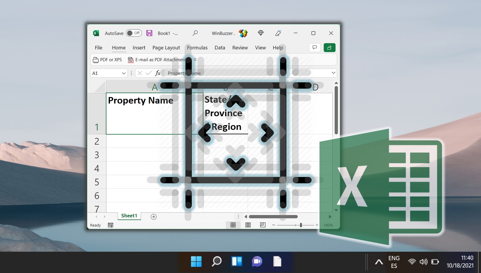
Extra: How to Wrap Text in Excel (Automatically and Manually)
Knowing how to wrap text in Excel is important so that your spreadsheet doesn't get any wider than it needs to be. The wrap text function in Excel lets you break text into multiple lines, therefore increasing the length of your cell. In our other guide, we show you how to wrap text in Excel, using both Excel line breaks and its automatic word wrap functionality.
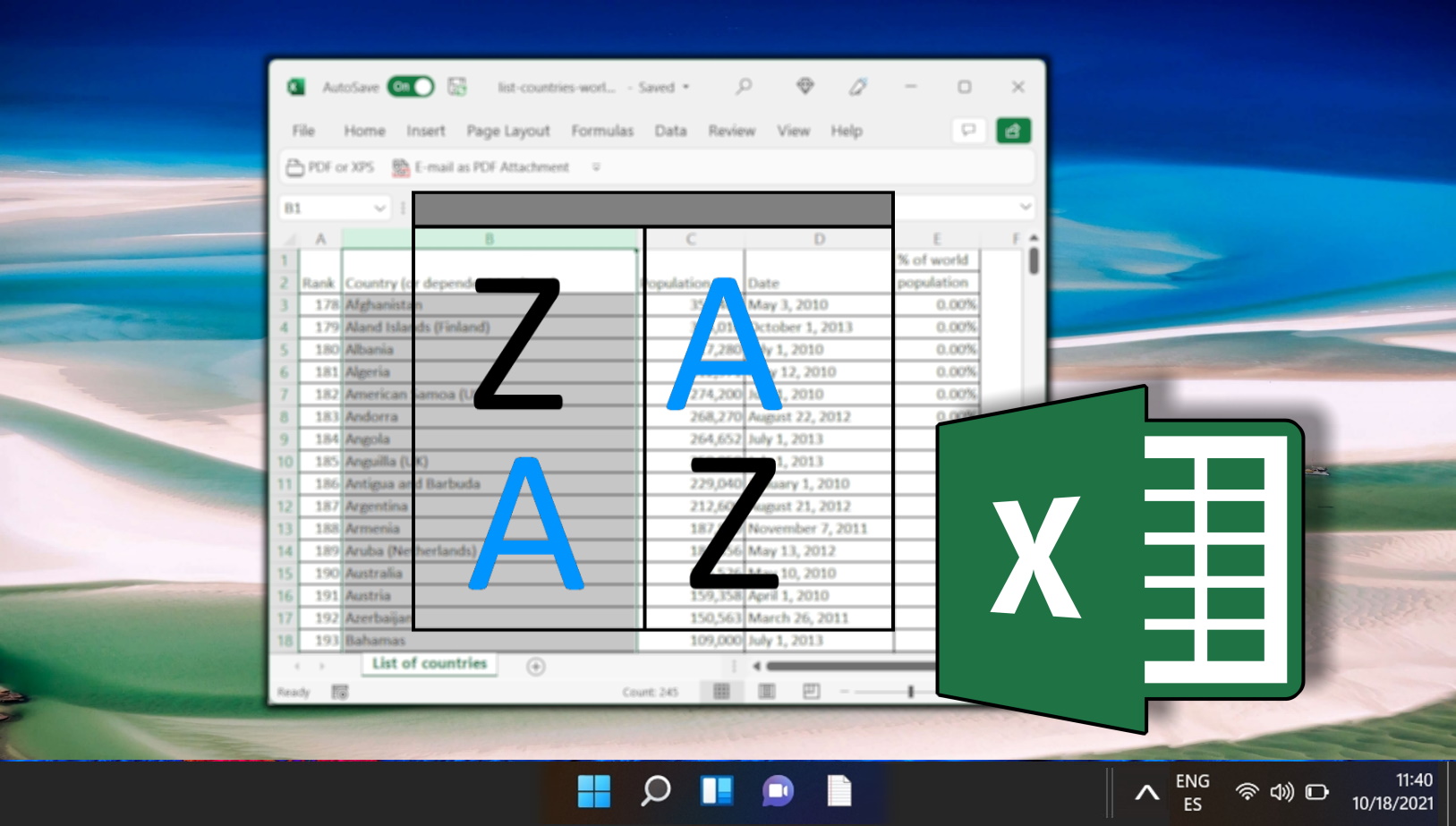
Extra: How to Alphabetize Data in Excel Columns or Rows
One of the most common types of sorting in Excel is alphabetical sorting. Whether it's a list of names, businesses, or mail addresses, sorting helps to organize and keep track of what you're doing. In our other guide, we are showing you how to alphabetize in Excel for both rows and columns.
Extra: How to Structure Collected Data in Excel
To make the most of Excel's features, you need to structure your data properly. Data structure refers to how you organize your data in a spreadsheet. A good data structure makes it easy to perform calculations, filter, and sort data, create charts and pivot tables, and apply formulas and functions. In our other guide, we show you how to structure collected data in Excel using some best practices and tips.

Last Updated on April 18, 2024 9:47 pm CEST by Markus Kasanmascheff