The ability to hide and unhide rows and columns in Excel is particularly useful for managing large datasets, protecting sensitive information, and maintaining a clean, focused workspace. This tutorial aims to guide you through the simple yet effective techniques of hiding and unhiding rows and columns in Excel, ensuring that you can control the visibility of your data with ease.
Why Hide Rows and Columns in Excel?
Hiding rows and columns in Excel is a common practice for several reasons. Firstly, it allows users to conceal sensitive data or complex formulas that are crucial for calculations but not necessarily needed for display. This is particularly important in shared workbooks where you want to prevent accidental modifications. Secondly, hiding irrelevant or less important data can help in focusing on the key information, making data analysis and presentation more efficient. Lastly, for large spreadsheets with extensive data, hiding unused rows and columns can significantly declutter the interface, making it easier to navigate and work with the visible data.
Unhiding: Revealing the Concealed Data
While hiding data is crucial for various reasons, the ability to unhide rows and columns is equally important. Whether you’re revisiting a section of your spreadsheet for review or need to update hidden data, Excel provides straightforward methods to unhide rows and columns. This functionality is essential for maintaining the integrity and completeness of your data, especially when dealing with complex spreadsheets where hidden data plays a key role in calculations and outcomes.
How to Hide Rows and Columns in Excel
The process for hiding rows and columns in Excel is essentially the same, with the only difference being the initial selection of either rows or columns. We’ll guide you through various methods using rows as the example, including keyboard shortcuts and menu options, to efficiently hide the data you don’t need to display.
- Select the Excel rows or columns you want to hide
Using Mouse Drag:
Rows: Click on the row number of the first row you want to select. Then, hold down the left mouse button and drag up or down to extend the selection to other rows.
Columns: Click on the column letter of the first column you want to select. Then, drag left or right while holding down the left mouse button to extend the selection to other columns.
Using Shift Key:
Rows: Click on the row number of the first row you want to select. Then, hold down the Shift key and click on the row number of the last row you want to include in your selection.
Columns: Click on the column letter of the first column you want to select. Hold down the Shift key and click on the column letter of the last column you want to include.
Selecting Non-Contiguous Rows or Columns:
Using Ctrl Key (Cmd on Mac):
Rows: Click on the row number of the first row you want to select. Then, hold down the Ctrl key (Cmd key on Mac) and click on the row numbers of any other rows you want to include in your selection.
Columns: Click on the column letter of the first column you want to select. Hold down the Ctrl key (Cmd key on Mac) and click on the column letters of any other columns you want to include.

- Method 1: Click “Home”, then “Cells” and “Format”

- Then select “Hide Rows” or “Hide Columns” under “Visibility”

- Method 2: Right-click the selected rows or columns and select “Hide”

- Method 3: Use a hotkey
To Hide Excel Rows: Press Ctrl + 9
To Hide Excel Columns: Press Ctrl + 0 (zero)

How to Unhide Rows and Columns in Excel
This section will demonstrate how to make hidden rows and columns visible again. The procedure for unhiding is similar to hiding, with a slight variation in the steps involved. We’ll cover different approaches to unhide rows and columns, ensuring that you can easily access your complete data whenever necessary.
- Method 1: Click “Home”, then “Cells” and “Format”

- Then select “Unhide Rows” or “Unhide Columns” under “Visibility”

- Method 2: Select the rows or columns before and after the hidden rows/columns

- Right-click the selected rows or columns and select “Hide”

- Method 3: Select the rows or columns before and after the hidden rows and use a hotkey
To Unhide Excel Rows: Press Ctrl + 9
To Unhide Excel Columns: Press Ctrl + 0 (zero)
- Method 4: Use a double click to unhide rows or columns
Hover over the rows or columns before and after the hidden rows/columns until the cursor shows a separator and double-click.

How to Unhide All Rows and Columns in Excel at Once
This part of the tutorial will teach you how to unhide all rows and columns simultaneously in Excel. This method is particularly useful when dealing with extensive data sets where multiple rows and columns are hidden, and individual unhiding would be time-consuming. We’ll explore the most efficient ways to restore full visibility to your entire spreadsheet with just a few clicks.
- Click on the button in the upper left corner to select the whole table

- Use the hotkey to unhide rows or columns
To Unhide all Hidden Rows: Press Ctrl + 9
To Unhide all Hidden Columns: Press Ctrl + 0 (zero)

How to Unhide Top Rows in Excel
Unhiding the top rows in Excel can sometimes be tricky, especially if they are the very first rows of the spreadsheet. This section is dedicated to showing you how to effectively unhide the top rows in your Excel worksheet. This method is particularly useful when the standard unhiding techniques don’t seem to work, as is often the case with the first few rows.
- Option 1 for selecting: Type “A1” in the Cell Name Box and press Enter
This action will move the selection to the specified cell, even if it’s in a hidden row.
If other top rows are hidden (say Row 2) type A2 (or the corresponding cell in the hidden row like A3, A4, etc.), to jump to the respective cell.
- Option 2 for selecting: Click “Home”, “Editing”, “Find & Select” and then “Go To”

- Put the cell name as “Reference” and click “OK”

- Use one of the methods described previously to unhide the row
Using the “hover and double-click method” before the first visible row number is generally a quick solution.
FAQ – Frequently Asked Questions About Hiding and Unhiding Rows/Columns in Excel
Can I set a default to always hide certain rows/columns when opening an Excel file?
By default, Excel doesn’t offer a direct feature to automatically hide specific rows/columns upon opening a file. However, a workaround involves saving the file with the desired rows/columns already hidden. For a more dynamic solution, you can use Visual Basic for Applications (VBA) to write a simple macro that hides specified rows/columns every time the workbook is opened. This requires basic knowledge of VBA scripting and can be done by accessing the Developer tab, opening the Visual Basic editor, and writing a macro in the ‘Workbook_Open’ event.
How can I protect hidden rows/columns from being unhidden by others?
To protect hidden rows and columns from being unhidden, you can use Excel’s sheet protection feature. Right-click the sheet tab, select “Protect Sheet,” and then choose the actions you want to allow users to perform. By setting a password, you ensure that only users with the password can unhide the rows/columns. Remember, this doesn’t encrypt the data, so it’s more about preventing accidental changes rather than securing sensitive information.
Can hidden rows/columns affect my calculations or charts?
Hidden rows and columns in Excel are still considered in calculations, charts, and pivot tables unless explicitly excluded. This means formulas that reference a range of cells will include the values in hidden cells. For charts, data in hidden rows/columns may still be displayed unless you adjust the chart data range or use filters to exclude the hidden data. To exclude hidden cells from some functions, you can use the SUBTOTAL function, which offers options to ignore values in hidden rows.
What’s the difference between hiding and grouping rows/columns in Excel?
Hiding rows/columns removes them from view without deleting the data, while grouping rows/columns allows you to collapse and expand a set of rows/columns to manage the visibility of large sections of data better. Grouping is particularly useful for creating an organized structure in your data, allowing users to quickly expand or collapse data sets to either view detailed information or get a summary. You can group rows/columns by selecting them, going to the Data tab, and clicking on “Group” in the Outline group.
How can I find if there are any hidden rows/columns in my sheet?
Hidden rows and columns can be identified by looking for breaks in the sequence of row numbers or column letters along the edges of the sheet. If you notice a row number or column letter skipping (e.g., from 4 to 6), it indicates that a row/column is hidden in between. Additionally, a slightly thicker line where the row or column is hidden might be visible. For a comprehensive check, you can select the entire sheet by clicking the corner button above row numbers and to the left of column letters, and then choose to unhide rows/columns from the context menu or the Home tab.
Can I hide rows/columns based on cell values or conditions?
Excel doesn’t provide a direct feature to automatically hide rows/columns based on cell values or conditions directly through the UI. However, you can achieve this using Conditional Formatting combined with a VBA script. The Conditional Formatting can visually indicate the rows/columns that meet certain conditions, and the VBA script can be written to automatically hide these rows/columns based on the formatting or specific cell values. This method requires basic knowledge of Excel’s VBA programming.
Is there a limit to the number of rows/columns I can hide in Excel?
Excel does not impose a specific limit on the number of rows/columns you can hide. You are limited only by the total number of rows and columns supported by Excel in your version (for example, Excel 2016 and later versions support up to 1,048,576 rows and 16,384 columns per sheet). However, excessive hiding of rows/columns can make navigation and data management cumbersome, so consider using grouping or filtering for better data management.
How do I ensure that hidden data remains confidential?
Hiding rows/columns is not a foolproof method to ensure confidentiality, as hidden data can easily be unhidden by any user. To secure sensitive data, consider using Excel’s cell protection features in combination with sheet protection to lock cells, and potentially workbook protection to secure the structure of the workbook. For higher security, consider encrypting the entire workbook with a password, which is available under the File > Info > Protect Workbook > Encrypt with Password option.
Why can’t I unhide certain rows/columns in Excel?
If you’re struggling to unhide rows/columns, it could be due to several reasons: the sheet might be protected, the rows/columns you’re trying to unhide may not be selected correctly, or there might be an issue with Excel itself. Make sure the sheet is unprotected by going to Review > Unprotect Sheet. To unhide rows, select the rows above and below the hidden ones; for columns, select the columns to the left and right. Then, right-click and choose “Unhide.” If problems persist, try closing and reopening Excel or checking for updates.
Can I hide multiple non-adjacent rows or columns at once?
Yes, you can hide multiple non-adjacent rows or columns by using the Ctrl key (Cmd key on Mac) to select them. After making your selection, right-click on one of the selected rows/columns and choose “Hide” from the context menu. This method allows you to selectively hide various parts of your worksheet without affecting adjacent rows/columns.
How do I hide rows/columns without losing data?
When you hide rows/columns in Excel, the data within them is not deleted or removed; it’s merely made invisible to provide a cleaner view of your worksheet. The data in hidden rows/columns continues to exist and can still be referenced in formulas and functions. To unhide them and make the data visible again, you need to select the rows/columns adjacent to the hidden ones and then use the “Unhide” option from the right-click context menu or the Home tab.
Can hiding rows/columns improve Excel’s performance?
Hiding rows/columns in Excel can make navigating and viewing your worksheet easier, but it has a minimal impact on the application’s performance. Excel still processes hidden data for calculations and other operations, so if you’re experiencing performance issues, consider other optimization techniques such as reducing file size, limiting the use of volatile functions, and minimizing the use of complex array formulas.
What keyboard shortcuts can I use for hiding and unhiding?
For quickly hiding rows, you can use the Ctrl + 9 shortcut. To hide columns, use Ctrl + 0. To unhide, you’ll need to first select the rows/columns surrounding the hidden area, but there’s no direct keyboard shortcut for unhiding. You’ll need to use the right-click context menu or the Home tab options after making the correct selection.
How can I troubleshoot issues when hiding/unhiding rows/columns?
If you encounter issues while trying to hide or unhide rows/columns, check a few things: ensure you’re not in the middle of editing a cell, as this can prevent certain actions; verify that the sheet isn’t protected, which would restrict hiding and unhiding; and ensure you’re selecting the rows/columns correctly (for unhiding, select the rows/columns on either side of the hidden ones). If none of these steps resolve the issue, restarting Excel or repairing the Office installation might help.
Is there a way to quickly hide every other row/column for readability?
Excel doesn’t have a built-in feature to automatically hide every other row/column, but you can achieve a similar effect for readability by applying banded rows or “zebra striping” using Conditional Formatting. This doesn’t hide rows/columns but changes their background color to improve readability. To apply banded rows, select your range, go to the Home tab, choose “Conditional Formatting,” then “New Rule,” and use a formula to format every other row.
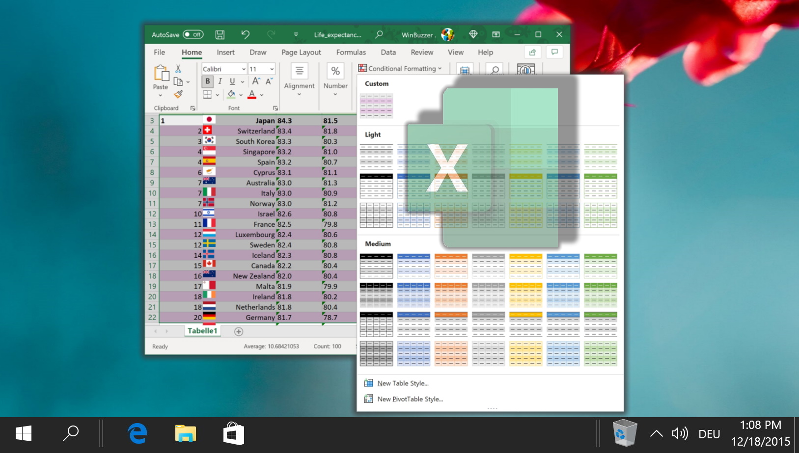
Extra: How to Add Shading to Alternating Rows in Excel
It’s an old trick at this point, but applying shading (zebra stripes) to alternative rows in Excel makes your sheet easier to read. The effect, also known as banded row, allows your eyes to keep their place more easily when you’re scanning a spreadsheet. The difficulty, then comes in knowing where to look and how to format cells as a table in the first place. In our other guide, we show you how to apply and customize table formatting to form alternating rows in Excel.
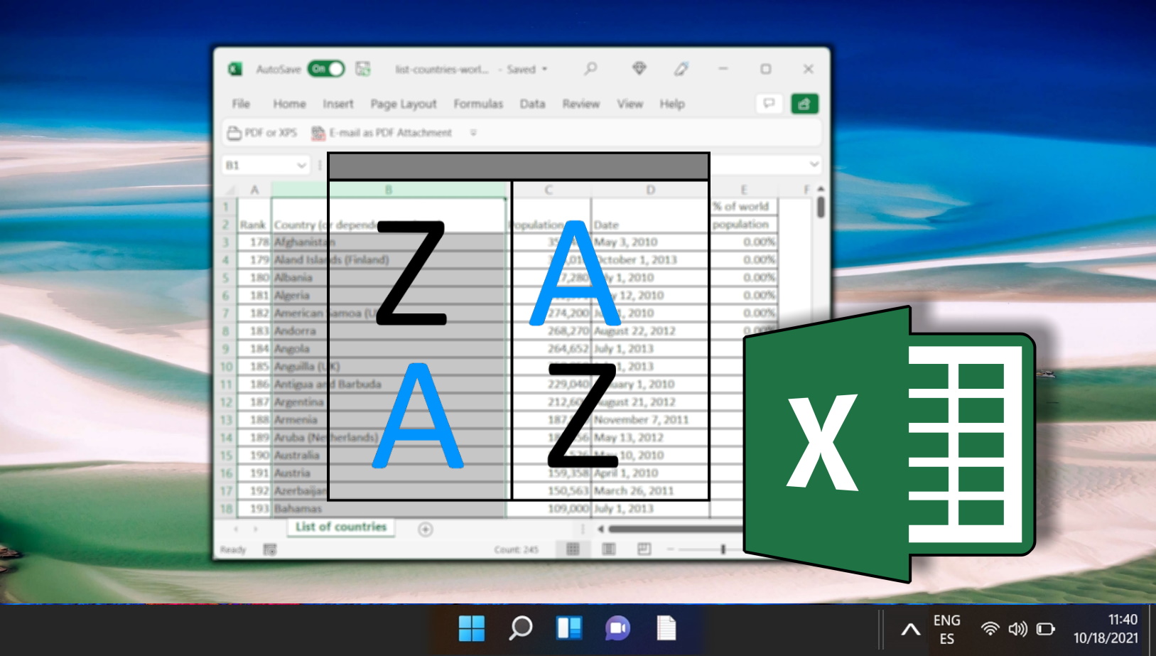
Extra: How to Alphabetize Data in Excel Columns or Rows
One of the most common types of sorting in Excel is alphabetical sorting. Whether it’s a list of names, businesses, or mail addresses, sorting helps to organize and keep track of what you’re doing. In our other guide, we are showing you how to alphabetize in Excel for both rows and columns.
Extra: How to Remove Table Formatting in Excel
In Excel, you can apply predefined table styles, making your data presentation-ready. However, there are instances where you might want to strip away the table formatting without losing the underlying data. In our other guide we show you various techniques to remove table formatting in Excel.

Extra: How to Structure Collected Data in Excel
To make the most of Excel’s features, you need to structure your data properly. Data structure refers to how you organize your data in a spreadsheet. A good data structure makes it easy to perform calculations, filter, and sort data, create charts and pivot tables, and apply formulas and functions. In our other guide, we show you how to structure collected data in Excel using some best practices and tips.