It can be beneficial in many situations to display the difference between two numbers as a percentage. Doing so helps to put a change into a more understandable format for the average reader. In this guide we show you how to calculate this percentage change in Excel using an Excel percentage formula.
The first thing you should know is that to calculate the percentage change between two numbers you must minus the new value from the old value, then divide it by the old value.
Need an example? Let’s say we made $2 in ad revenue from an article in June. In July, there was a big increase traffic, leading to $7 in revenue. We would calculate percentage change like so: (7 - 2) ÷ (2) = 2.5 * 100 = 250%.
At this point, we should note that there is a difference between percentage change and percentage difference. Percentage change is used to calculate the difference between an old and new value.
Percentage difference is used when both values are from similar time periods or origins. Therefore, you divide by the average of the two values rather than the difference between them.
How to Calculate Percent Change in Excel
This section will guide you through calculating the percentage change between two values in Excel. This is a crucial skill for anyone looking to analyze changes in data over time, providing a clear and understandable way to present growth, decline, or trends.
- Create a New Column for Percentage Change
Click the cell to the right of the two numbers where you will enter your percentage change formula. This step is essential for organizing your Excel sheet and clearly displaying the percentage change between the old and new values.

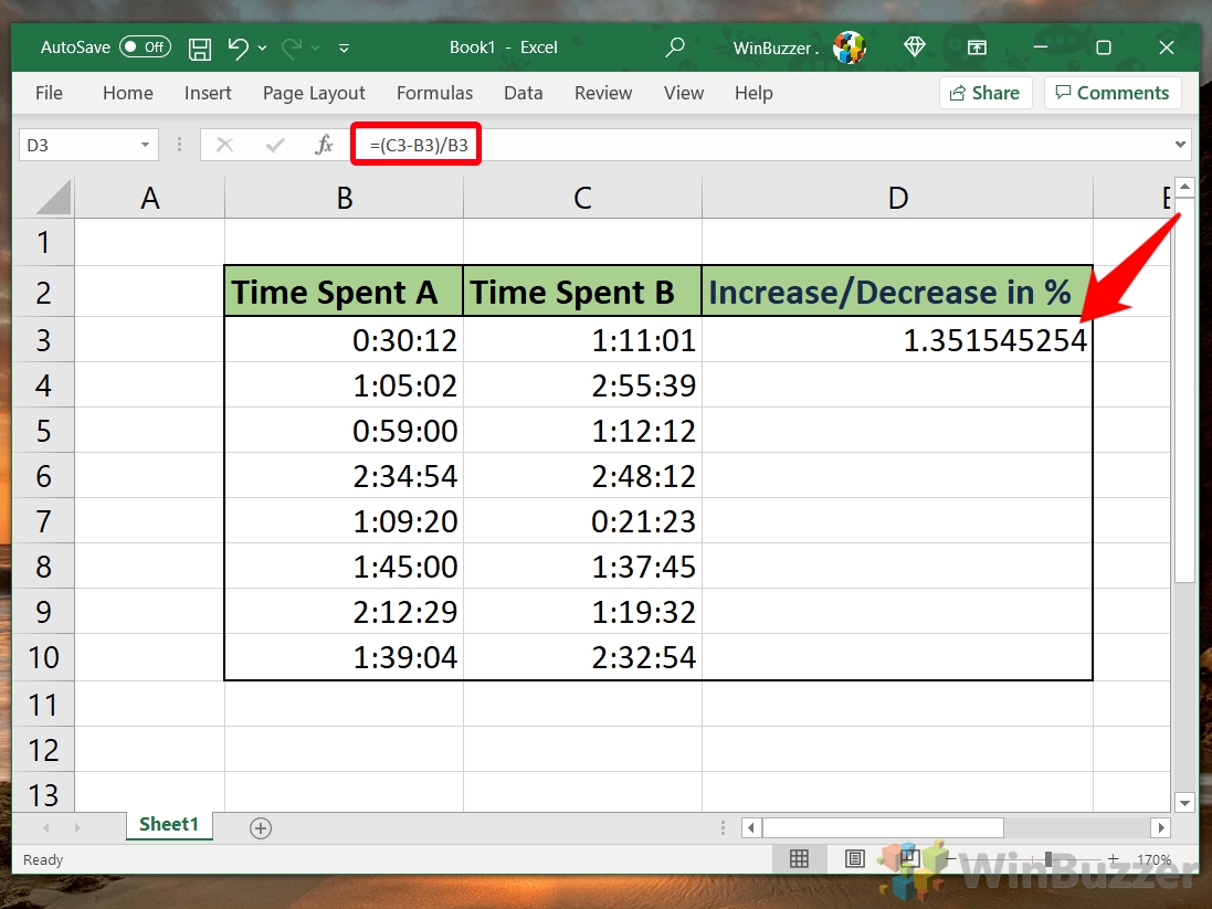
- Enter the Percentage Change Formula
Type the formula=(old value's cell - new value's cell)/new value's cellinto the selected cell. For instance, if your old value is in cell B3 and your new value is in cell C3, you would enter=(C3-B3)/B3. This formula calculates the difference between the two values, divides it by the old value, and prepares it for conversion to a percentage format, initially displaying as a decimal.
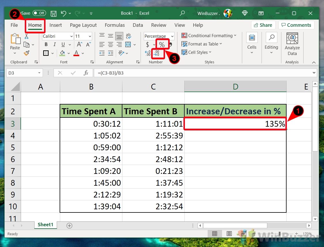
- Change Cell Formatting to Percentage
With the cell still selected, go to the “Home” tab in the Excel ribbon and click the “%” icon, then adjust the decimal points using the “.00->.0” option.The first will format your value as a percentage by multiplying the number by 100 and adding a percent symbol. The second will reduce the number of decimal points by one. You can press this multiple times, or the “.0 <-.00” button next to it to adjust the decimal points to your liking.
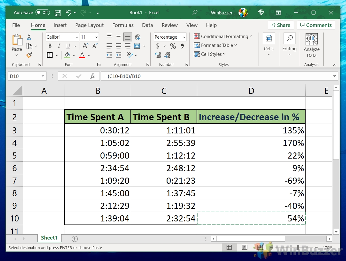
- Apply the Excel Percentage Formula to Additional Rows
Drag the small square at the bottom-right corner of your formatted cell down to cover all relevant rows. This automates the calculation process for each row, ensuring consistency across your data set and saving you time.
FAQ – Frequently Asked Questions About Excel Percentage Calculations
Can I use conditional formatting to highlight significant percentage changes in Excel?
Yes. To use conditional formatting for highlighting cells that represent significant percentage changes, first select the cells with your percentage change calculations. Go to the “Home” tab, click “Conditional Formatting,” and choose “Highlight Cells Rules“. Select a rule, such as “Greater Than” or “Less Than“, and enter the value that defines “significant” for your analysis. For instance, input “10” to highlight changes greater than 10%. Finally, choose a formatting style from the available options, and click “OK“. This feature is particularly useful for quickly identifying outliers or significant trends in your dataset.
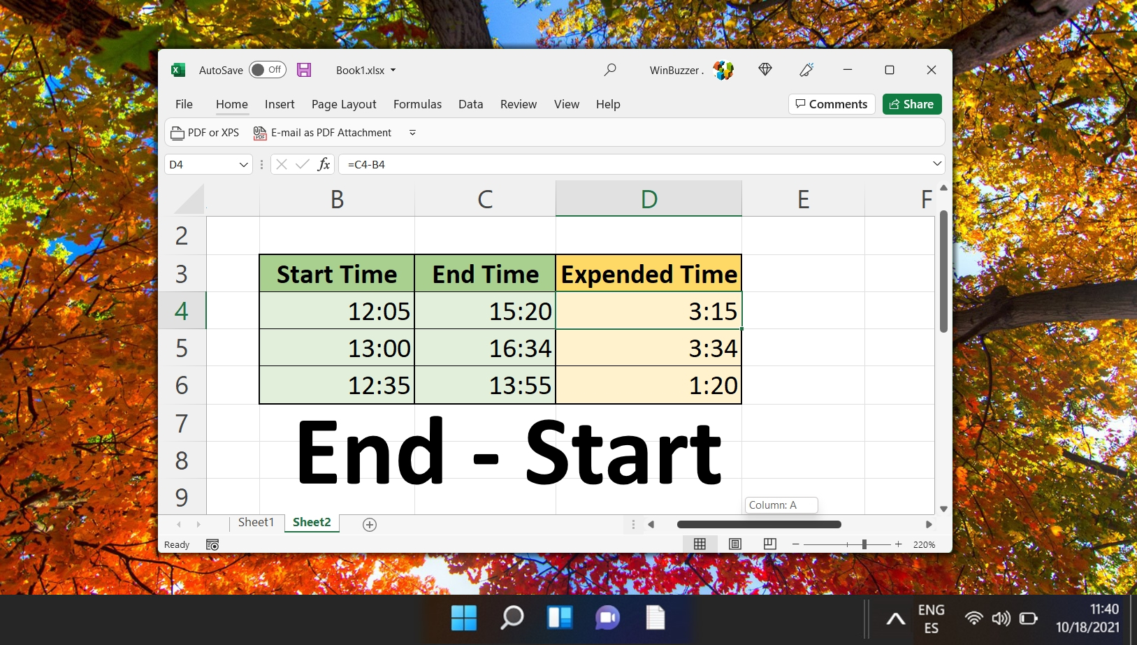
What if my values are in different sheets? Can I still calculate the percentage change?
Definitely. When your data points (old value and new value) are located on different sheets, you can still calculate the percentage change by properly referencing these cells across sheets. To reference a cell in a different sheet, use the format SheetName!CellNumber in your formula. For example, if your old value is in cell A1 on Sheet1, and your new value is in cell A1 on Sheet2, your formula in the cell where you want to show the percentage change (on either sheet) would be =(Sheet2!A1-Sheet1!A1)/Sheet1!A1. Remember to format the result as a percentage for clarity.
How can I display negative percentages in red in Excel?
Using Conditional Formatting, you can visually distinguish negative percentages by displaying them in red. Select the range of cells with your percentage change calculations. Head to the “Home” tab and click “Conditional Formatting“, then choose “New Rule“. Select “Format only cells that contain“, set the rule to “Cell Value” “less than” and enter “0” in the value box. Click “Format“, select the “Font” tab, choose the red color, and press “OK“. Complete the setup by again clicking “OK” in the New Formatting Rule dialog. This will automatically turn any negative percentage values in your selected range red, making them easily identifiable.
Is it possible to automate percentage change calculations for dynamic data ranges in Excel?
Yes, automating percentage change calculations for dynamic data ranges can be achieved by creating a dynamic named range with the OFFSET function or using Excel tables. For dynamic named ranges, use the OFFSET function combined with COUNTA to reference your data range dynamically, adjusting automatically as you add or remove data. Once your dynamic range is set up, apply the percentage change formula to this range. When using Excel tables, your formulas can reference table columns directly and will automatically adjust as new rows are added. This is an efficient way to manage data that frequently changes in size.
How do I reverse the percentage change formula to find the original value?
To find the original value before a percentage change when you know the new value and the percentage change, you can rearrange the initial formula. If you have a percentage increase, use Original Value = New Value / (1 + Percentage Change). For a percentage decrease, use Original Value = New Value / (1 – Percentage Change). Ensure the percentage change is in decimal form for this calculation (for example, 20% becomes 0.2). This is particularly useful in financial analysis and projections where you might know the final amount and the percentage of growth or reduction but need to calculate the starting amount.
Can I use the percentage change formula for financial data analysis in Excel?
Absolutely. The percentage change formula is vital in financial analysis for a variety of applications, including calculating growth rates, evaluating return on investments, assessing profit margins, and comparing financial metrics over different time periods. By providing a clear measure of how values have increased or decreased relative to their starting points, it allows analysts to gauge performance, identify trends, and make informed decisions. For precise analysis, ensure your data is accurate and your formula is correctly applied, considering the specific context of your financial analysis.
What is the best way to visualize percentage changes in Excel?
To effectively visualize percentage changes in Excel, consider using charts that best represent your data’s nature and the insights you wish to convey. Line charts are ideal for showcasing trends over time, allowing viewers to track percentage changes across multiple data points. Bar or column charts are great for comparing percentage changes across different categories or groups at a single point in time. For more detailed analysis, consider using a combination of charts, such as overlaying a line chart on a bar chart, to provide a more nuanced view of your data. Always ensure your charts are clearly labeled and include a legend if necessary, to make them easily understandable.
How can I ensure my percentage change calculation ignores zero or blank cells?
To prevent your percentage change calculations from being skewed by zero or blank cells, incorporate an IF function to specifically handle these cases. For example, you might use =IF(OR(B1=0, B1=””, C1=0, C1=””), “”, (C1-B1)/B1) in your formula. This checks if either the old value (B1) or the new value (C1) is zero or blank and returns an empty string (“”) if true, otherwise, it calculates the percentage change. This approach ensures that your calculations are only performed on valid data, maintaining the integrity of your analysis.
Can the percentage change formula be used for time series data analysis?
Yes, the percentage change formula is instrumental in time series data analysis, as it helps identify growth, shrinkage, or trends within a data set over sequential time intervals. This analysis is vital in fields like economics, finance, weather forecasting, and more. To use it effectively, calculate the percentage change for each time interval compared to its predecessor. This will give you a clear view of how the data evolves over time, potentially uncovering seasonal patterns, growth trends, or alarming fluctuations that might not be immediately apparent from raw data alone.
Is there a way to calculate cumulative percentage change in Excel?
Calculating cumulative percentage change involves understanding the compounded effect of percentage changes over multiple periods. It’s not as straightforward as summing percentages but involves a multi-step calculation. Start by adding 1 to each individual percentage change (converted to decimal), then multiply all these adjusted values together. Finally, subtract 1 from this product and convert it back to a percentage. This gives you the overall cumulative effect of the changes over time on the initial value. This calculation is especially useful in investment analysis, where you might need to assess the compounded return over several periods.
How can I convert a series of percentage changes into a single cumulative figure?
Converting a series of individual percentage changes into a single cumulative figure involves calculating the compounded effect of all changes. First, convert each percentage change to its decimal form and add 1 to each. Multiply these adjusted values to get a single multiplicative factor for the entire series. Subtract 1 from this final product and then convert it back to a percentage to get the overall cumulative percentage change. This approach is valuable for understanding the total effect of sequential changes on an initial value, such as the compounded annual growth rate (CAGR) of an investment over multiple years.
Can Excel convert decimal changes to percentage changes automatically?
While Excel doesn’t automatically interpret decimal changes as percentage changes directly, you can quickly format any number as a percentage. Simply enter your calculation resulting in a decimal, select the cells you wish to format, and then click the “%” icon in the “Home” ribbon. This multiplies the decimal by 100 and displays the result with a percentage sign, making the interpretation of decimal changes as percentages straightforward and visually consistent.
What are the shortcuts to apply percentage formatting in Excel?
To quickly apply percentage formatting to selected cells in Excel, you can use keyboard shortcuts to streamline the process. After selecting your cells, you can press Ctrl+Shift+%. This instantly applies the percentage format to your selected data, making fast work of converting decimal numbers into percentages without navigating through the menu options.
How do I adjust the decimal places in my percentage results?
After you’ve converted your results to percentage format, you might want to adjust the number of decimal places to suit your reporting or analysis needs. Select the cells containing your percentage results, then use the “Increase Decimal” or “Decrease Decimal” buttons under the “Home” tab in the Excel ribbon to adjust the precision of your displayed percentages. This allows you to present your data more clearly, matching the level of detail that is most appropriate for your audience or analytical requirements.
Can I calculate percentage change between more than two periods in Excel?
Yes, you can calculate the percentage change across multiple periods by applying the percentage change formula between each pair of consecutive values in your series. This approach enables you to track the evolution of percentage change over time, revealing more intricate trends or patterns. It’s particularly useful in longitudinal studies or projects where understanding the progression or trajectory of change is essential. For a comprehensive analysis, consider using a pivot table or dynamic formulas to efficiently manage and analyze your time series data.
Related: How to Subtract in Excel (Numbers, Dates, Time, Percentages)
We all need to subtract numbers at one point or another, but sometimes a calculator just won’t cut it. In our other guide, we show you how to subtract in Excel? In our other guide, we show you everything you need to know, from subtracting numbers to text, dates, columns, percentages, and negative numbers.
Related: How to Square Root in Excel
Though Excel is most commonly used to perform simple addition and multiplication, it has all the functionality of a calculator and more. In our other guide, we show you how to find the square root of a number in Excel using three separate formulas.
Related: How to Use Alternating Rows in Excel
It’s an old trick at this point, but applying shading (zebra stripes) to alternative rows in Excel makes your sheet easier to read. The effect, also known as banded row, allows your eyes to keep their place more easily when you’re scanning a spreadsheet.
Related: How to Hide and Unhide Rows and Columns in Excel
The ability to hide and unhide rows and columns in Excel is particularly useful for managing large datasets, protecting sensitive information, and maintaining a clean, focused workspace. Our other tutorial shows you how to hide and unhide rows and columns in Excel, ensuring that you can control the visibility of your data with ease.